Tutorial
This step by step tutorial demonstrates how to:
Load and create configurations
Model stereotaxic frames
Add and register brain atlases based on the location of anatomical landmarks sampled on a subject when no MRI or CT scans are available.
Add and register assets such as meshes used for acoustic simulations domain definitions
Run k-wave simulations and grab the results for further analysis
Note
The complete configuration file for this demo is included under coperniFUS/examples/assets/Dual arms FUS + rec electrode rat tutorial config.json.
1. Launch CoperniFUS, load and create configurations
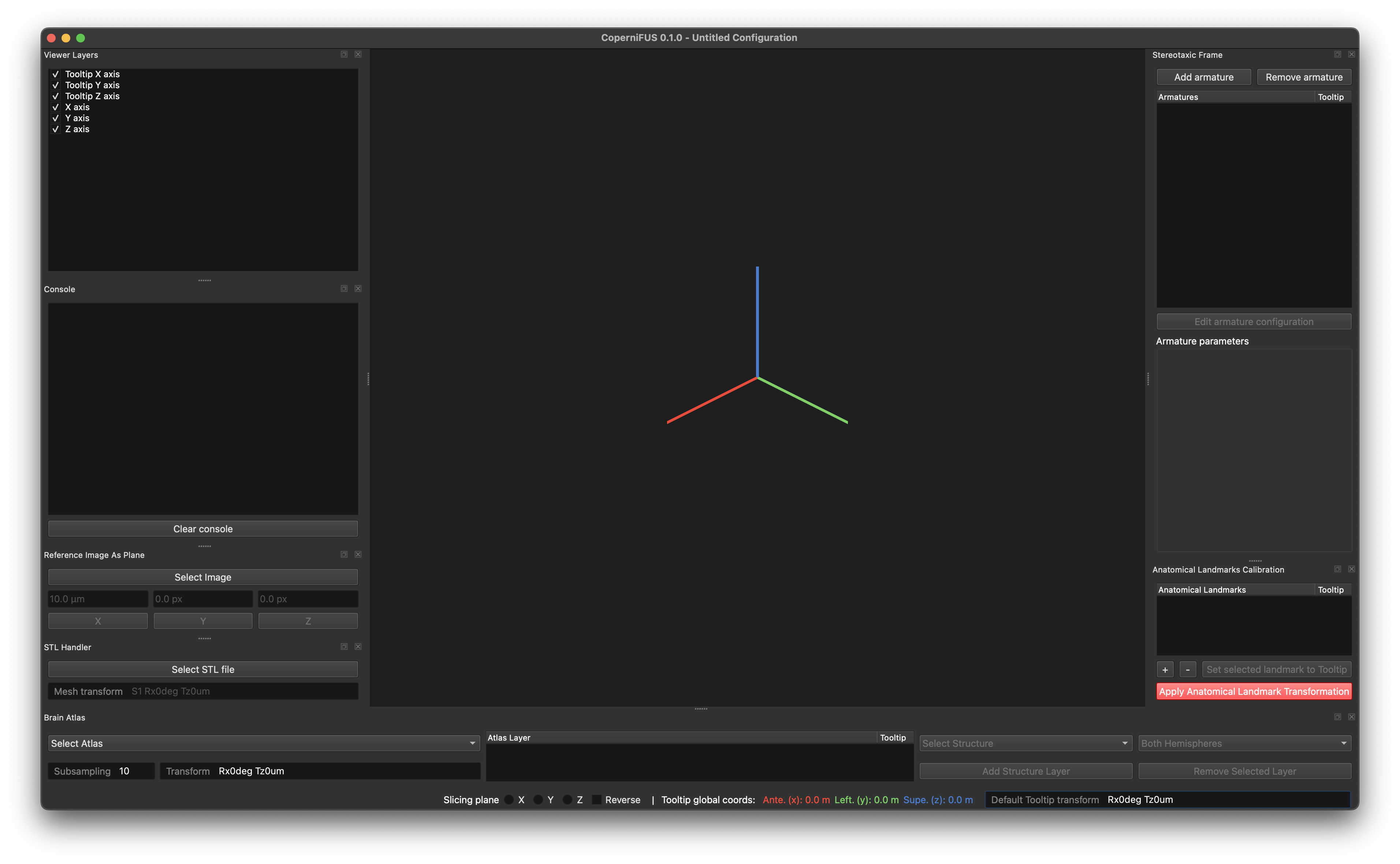
Open CoperniFUS by running coperniFUS in a terminal (or use it in interactive mode as described in Usage). If no configuration file exist, an empty viewer sill open.
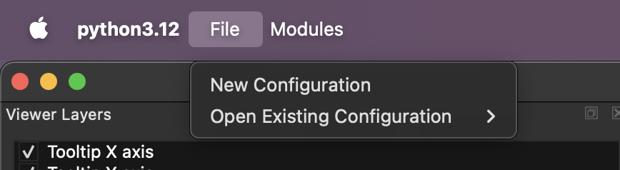
Create or open configuration files from the File menu
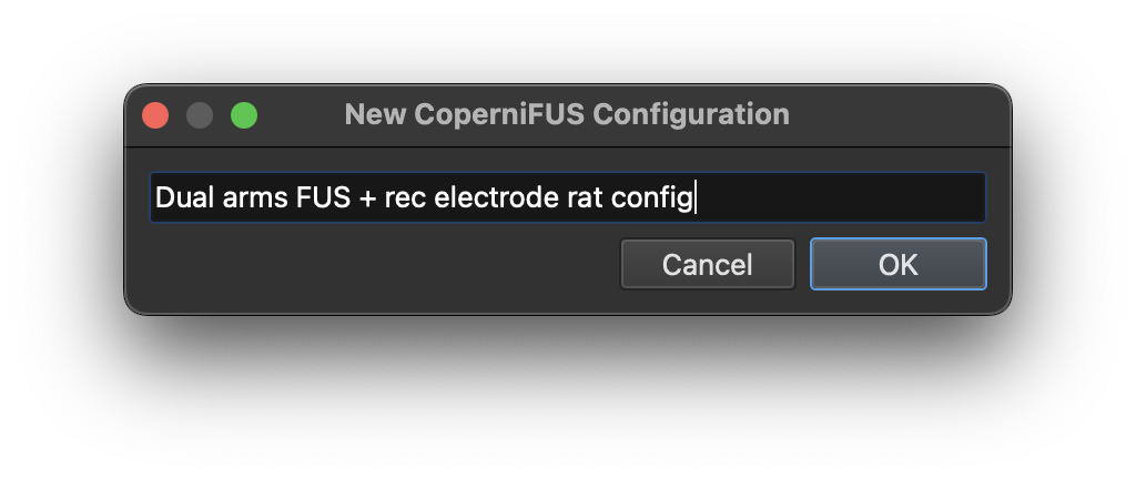
For the sake of this tutorial select New Configuration and input a name.
2. Add brain atlases
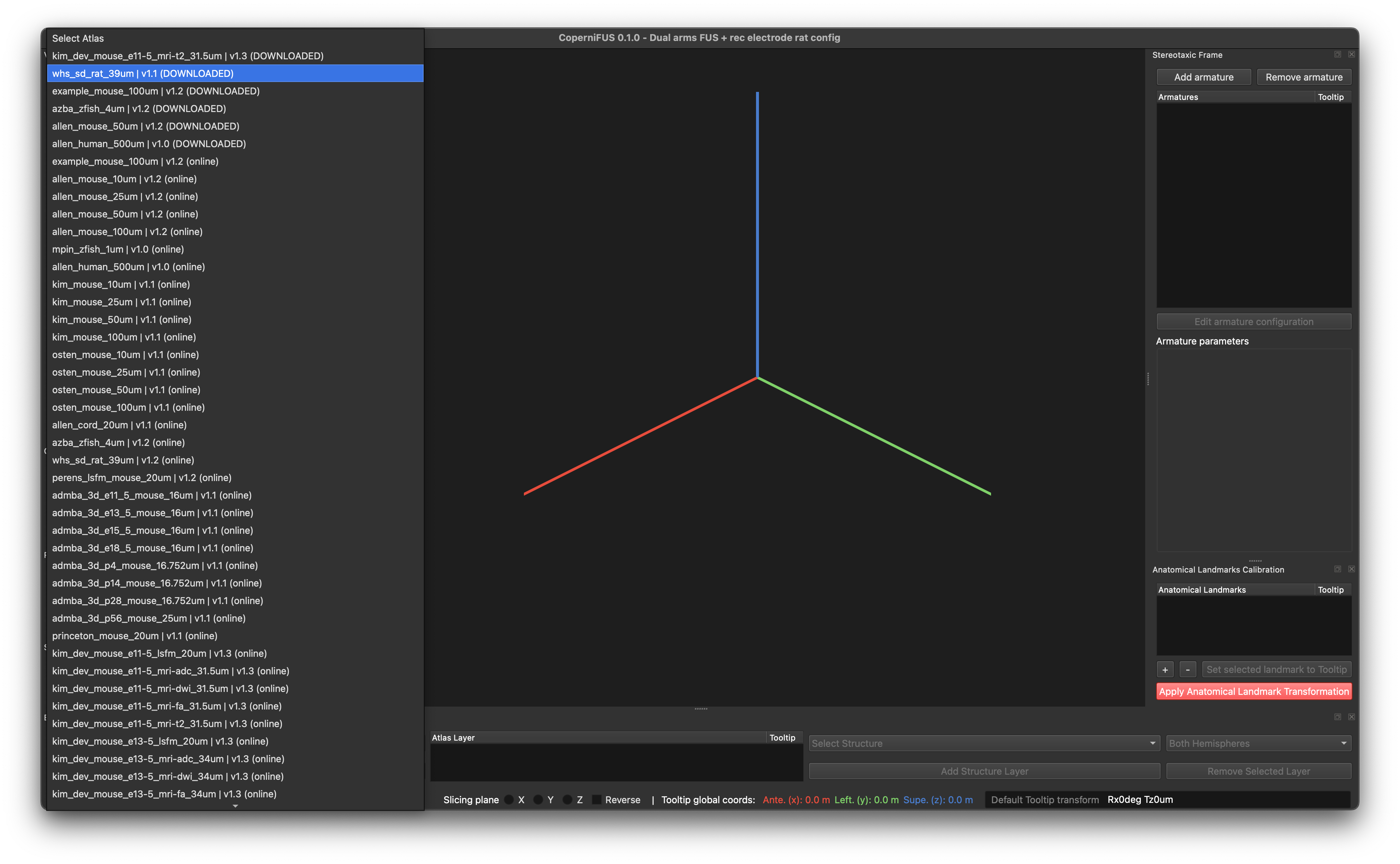
Add a brain atlas by selecting one in the Brain Atlas module.
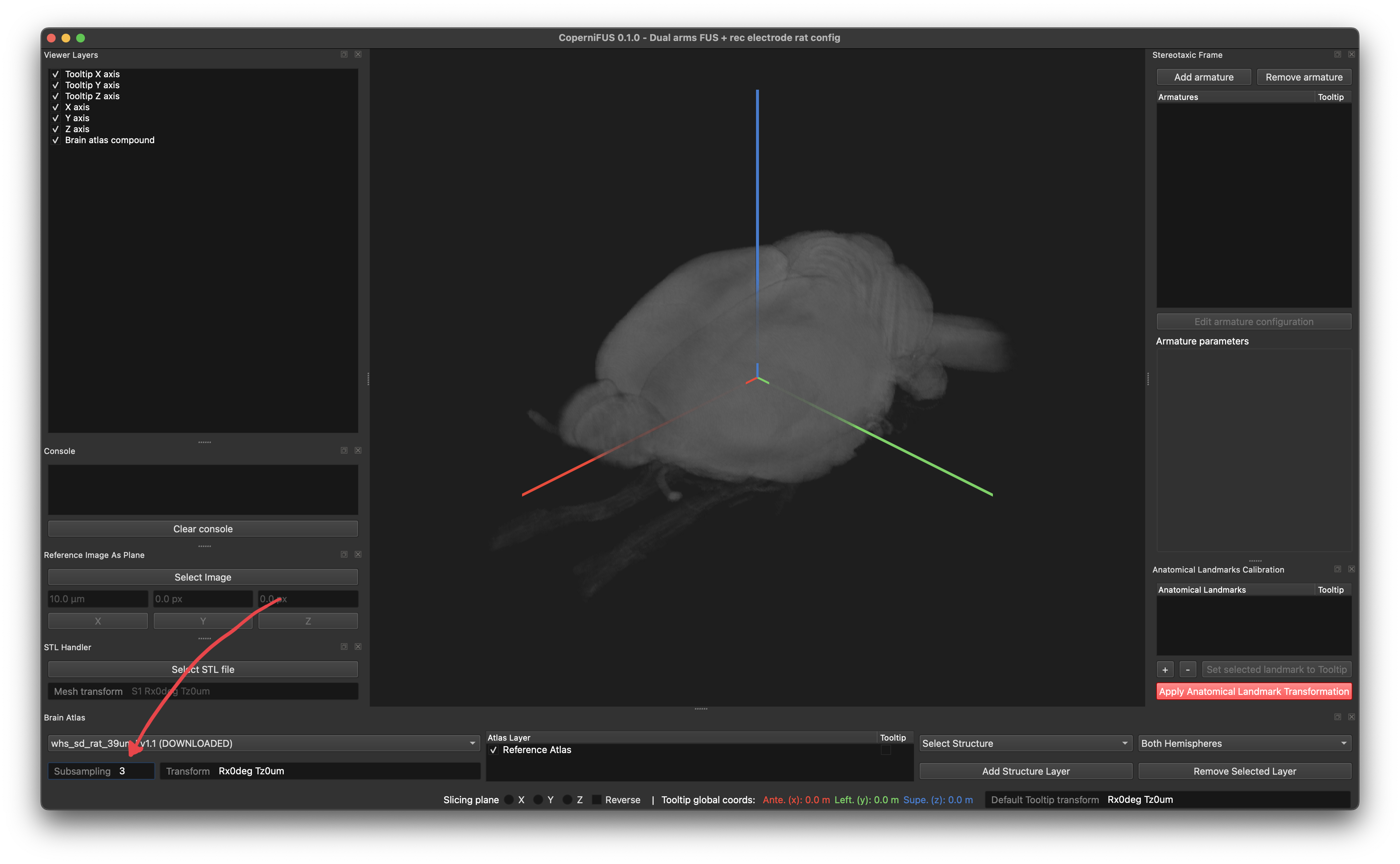
Note
To balance rendering performances and accuracy, an atlas subsampling factor can be adjusted.
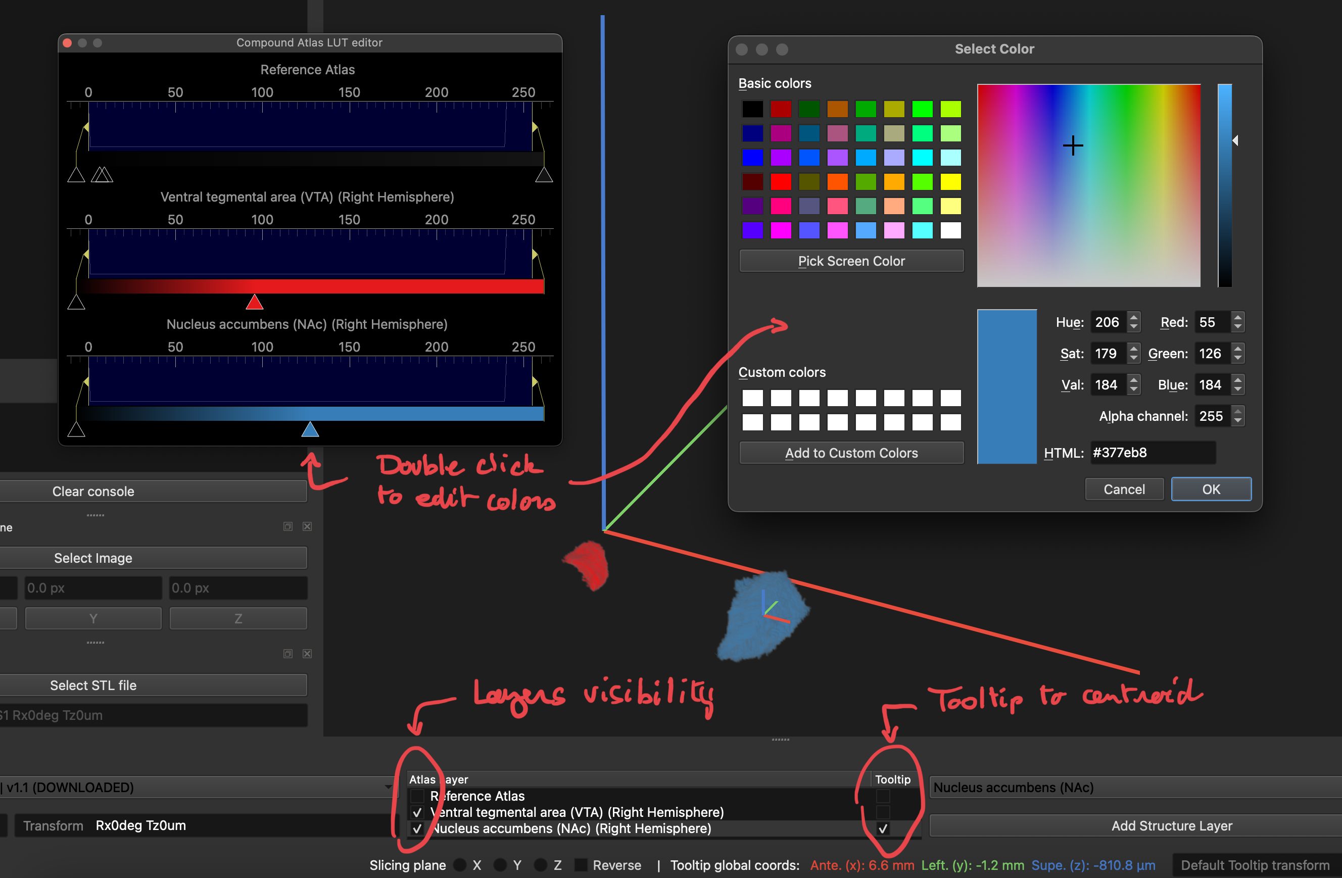
Brain structures layers can be added to the viewer.

Double clicking on the list of loaded layer allows the edition of their color and opacity. The Tooltip location can also be set to the centroid of structures assess their location.
3. Anatomical registration of atlases and assets
In the context of studies where access to MRI or CT scans is not possible, CoperniFUS enable the manual registration of atlases and assets such as skull meshes that can be used for acoustic simulations using k-Wave Python. Based the registration of anatomical landmarks, atlases and assets can be automatically transformed to better fit the anatomy of subjects.
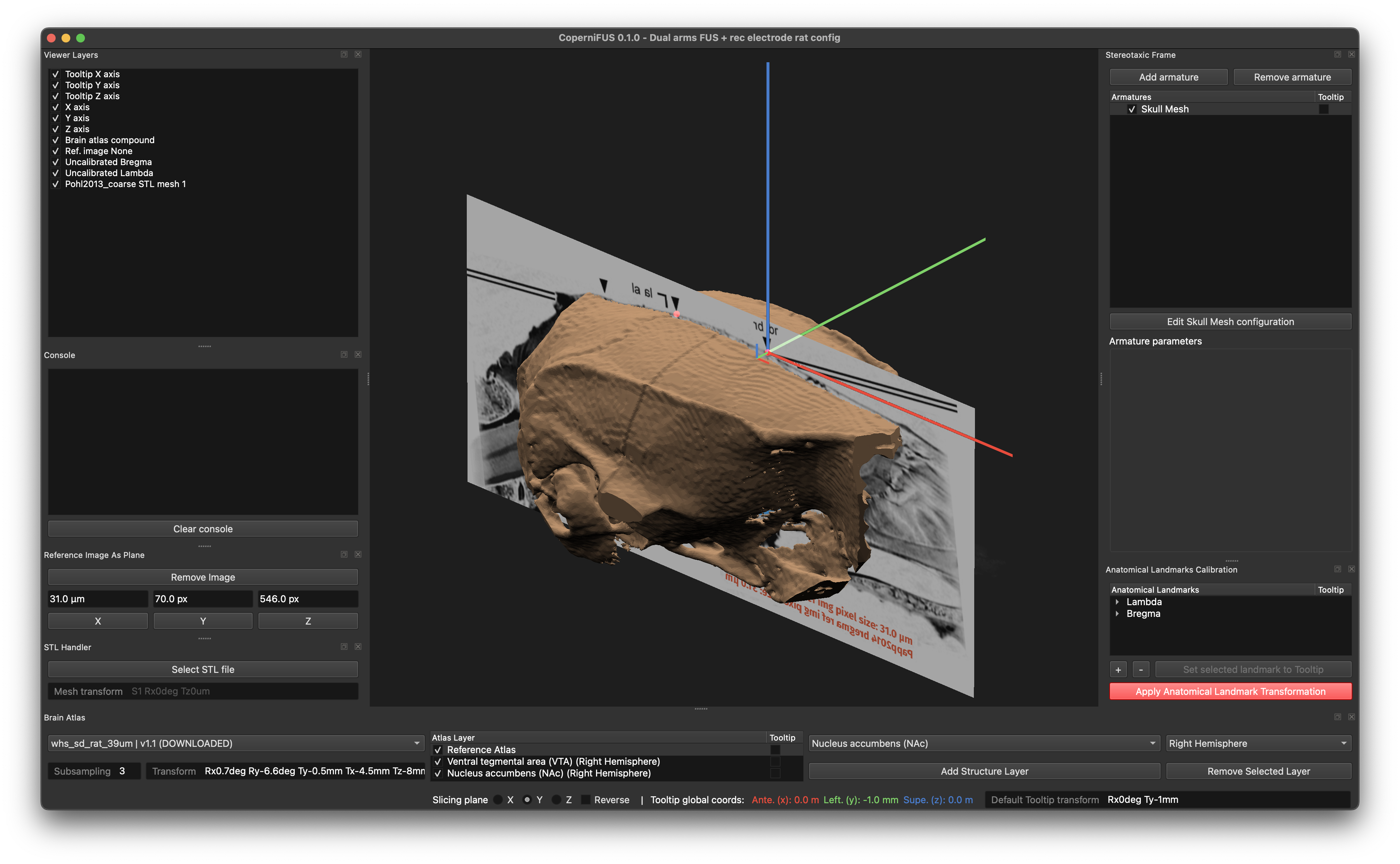
In this example, the Bregma landmark will be used ad the origin of the coordinate system. A reference image from the literature [Papp2014] is used register the Altas and skull meshes relative to its location. Using the Reference Image as Plane module, the image (available in the example/assets folder) can be loaded in the viewer. Click on Y to set the plane normal and adjust the pixel size and origin in pixel coordinates.
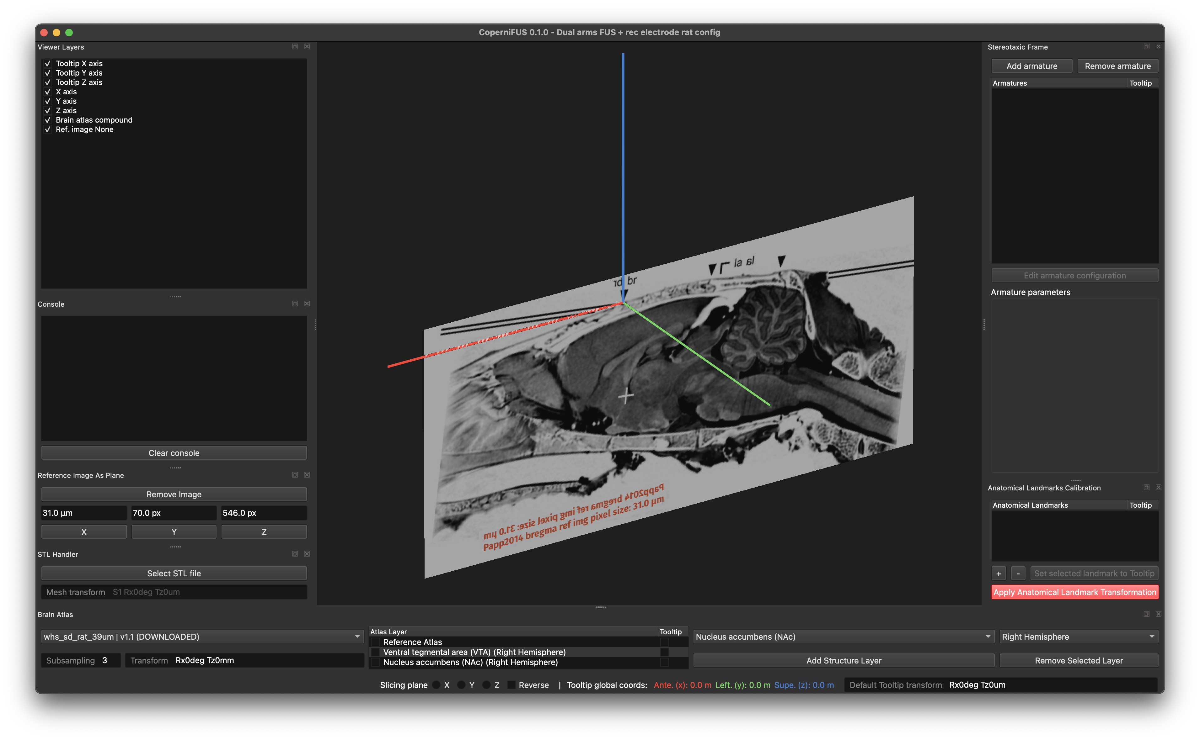
To simplify the initial atlas registration procedure, its color can be altered using the aforementioned editor.
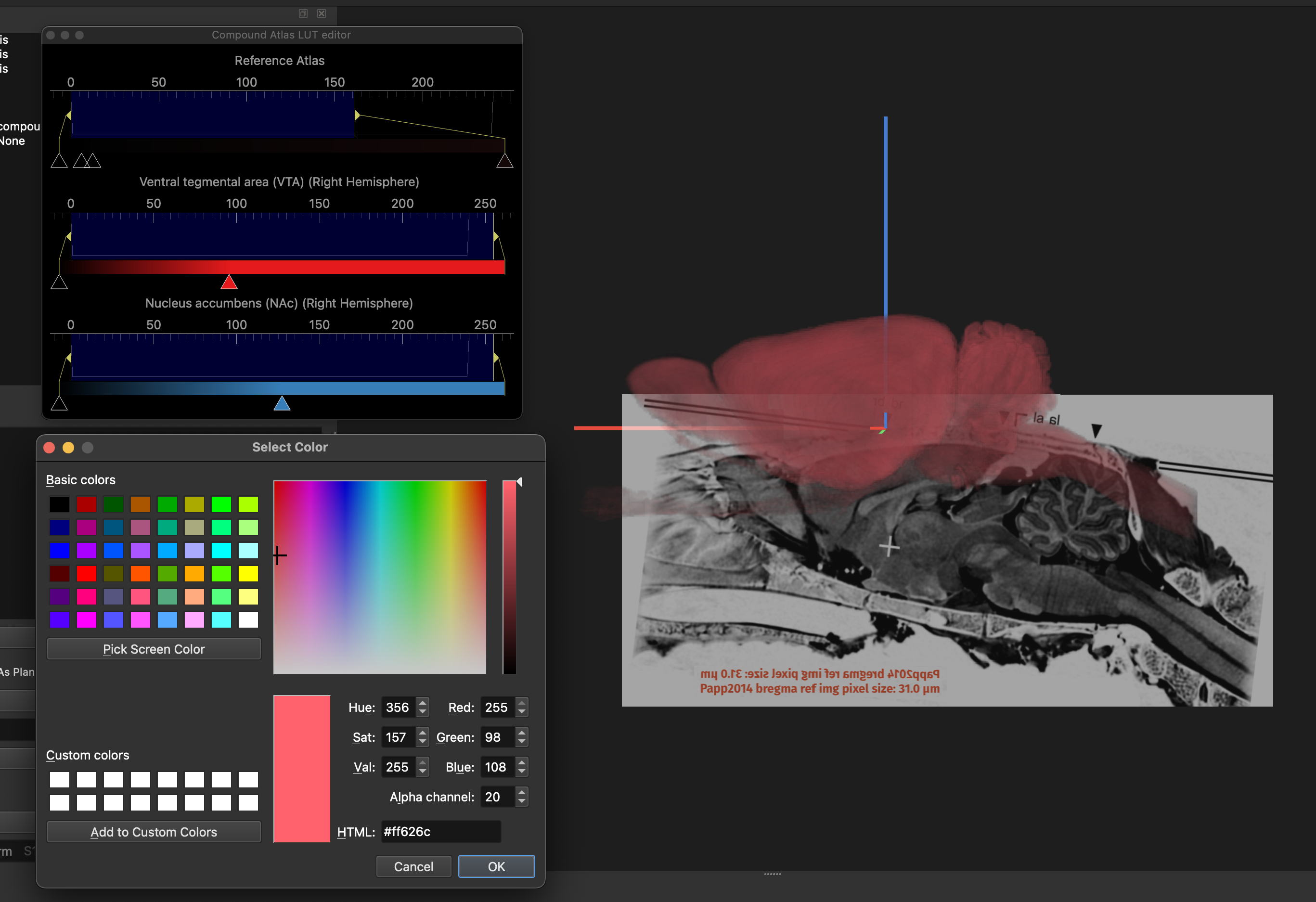
The location of the atlas is adjusted using the Transform editor of the Brain Atlas Module. The syntax for these affine transformations used throughout the software is detailed in Affine transformations as string syntax
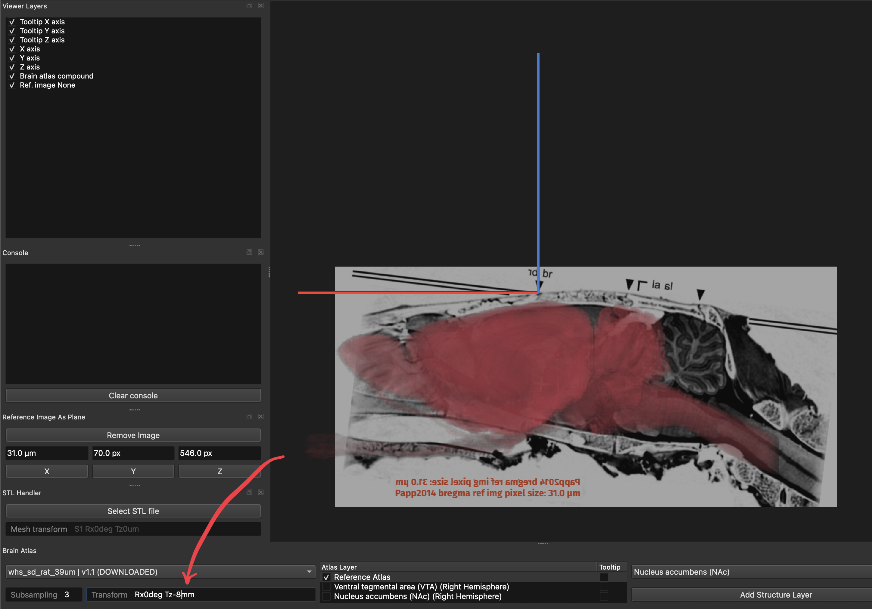
In this example, the required sequence of transformations was found to be Rx0.7deg Ry-6.6deg Ty-0.5mm Tx-4.5mm Tz-8mm .
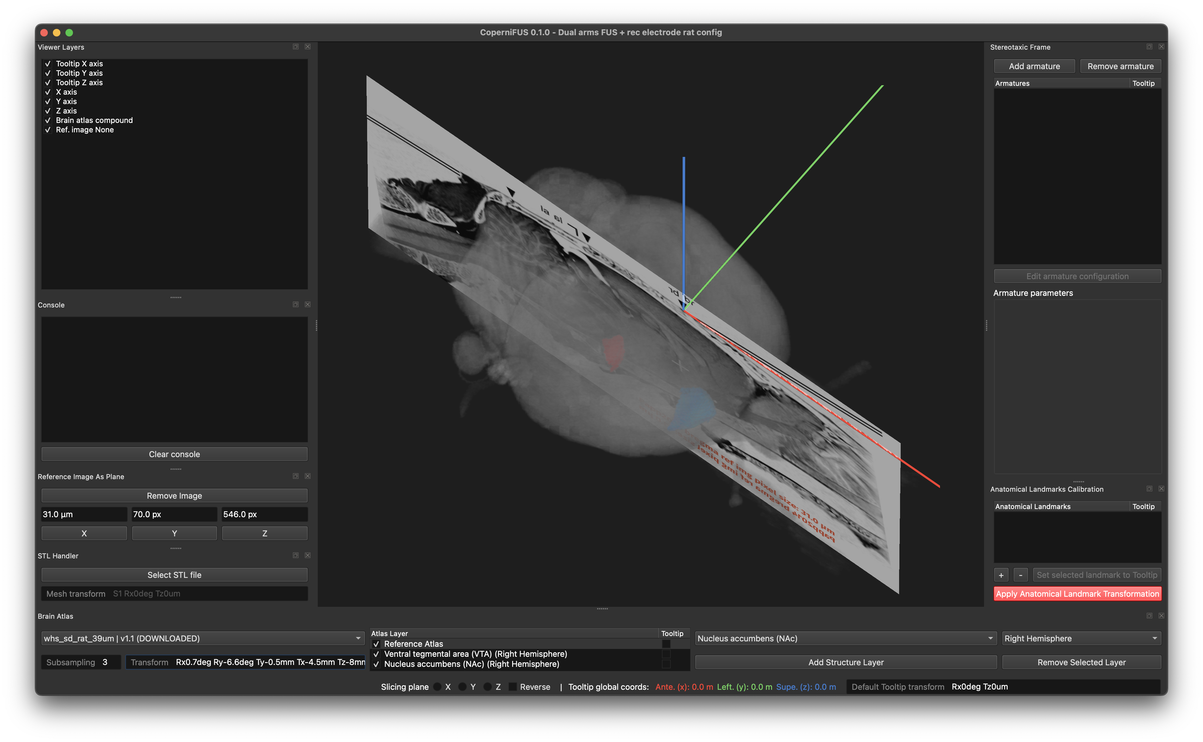
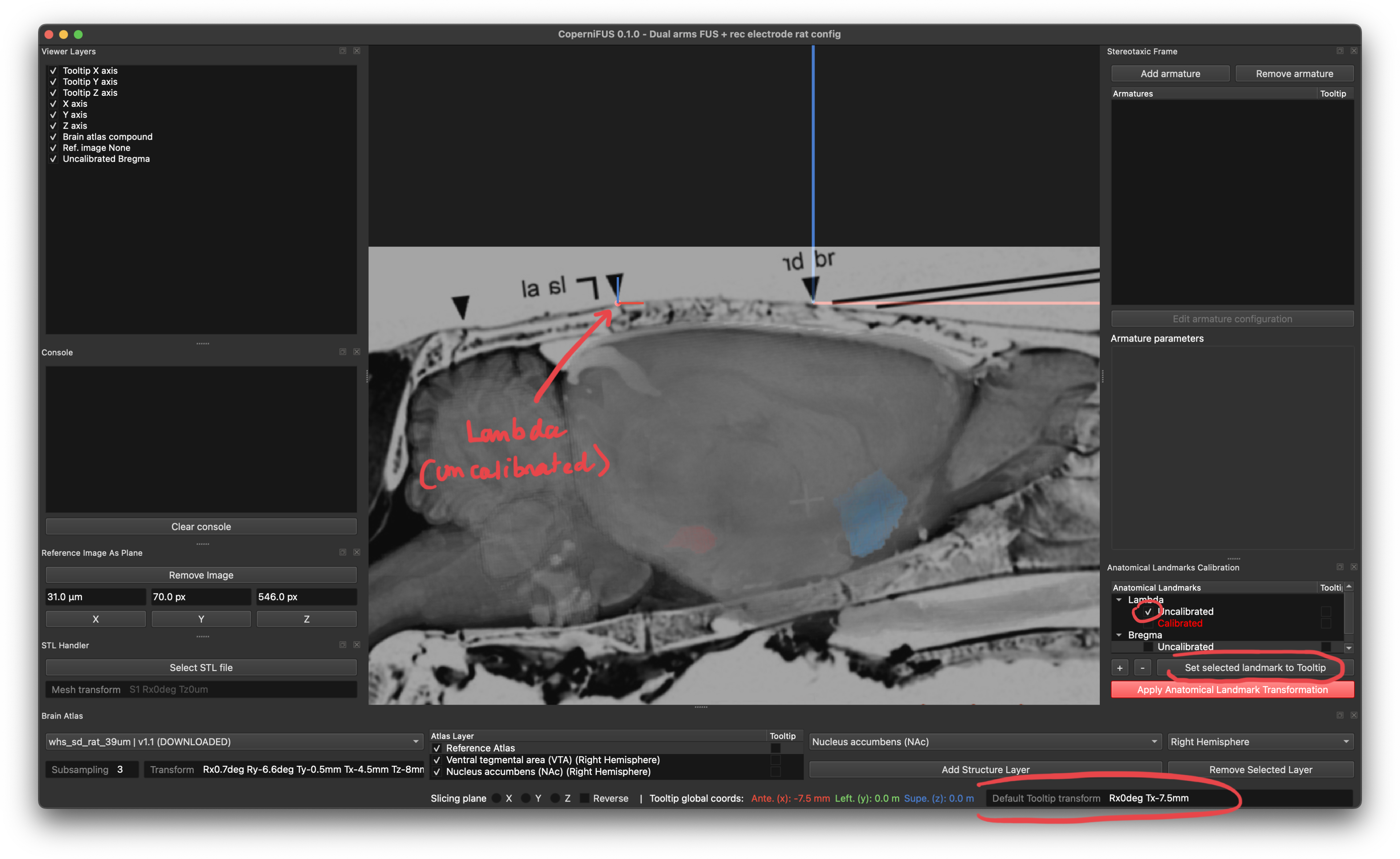
At this point the registration of uncalibrated anatomical landmarks used for calibration can be performed. Lambda and Bregma landmarks will be used, to start, add two landmarks in the Anatomical Landmarks Calibration module and set their names.
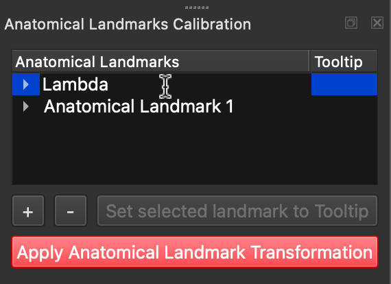
Coordinates can be set by unfolding the landmarks lists and selecting one element. Move the Tooltip to the appropriate location and click on Set selected landmark to Tooltip. Selected uncalibrated landmarks will appear as red dots in the viewer. As we will see later, calibrated ones are shown in green.
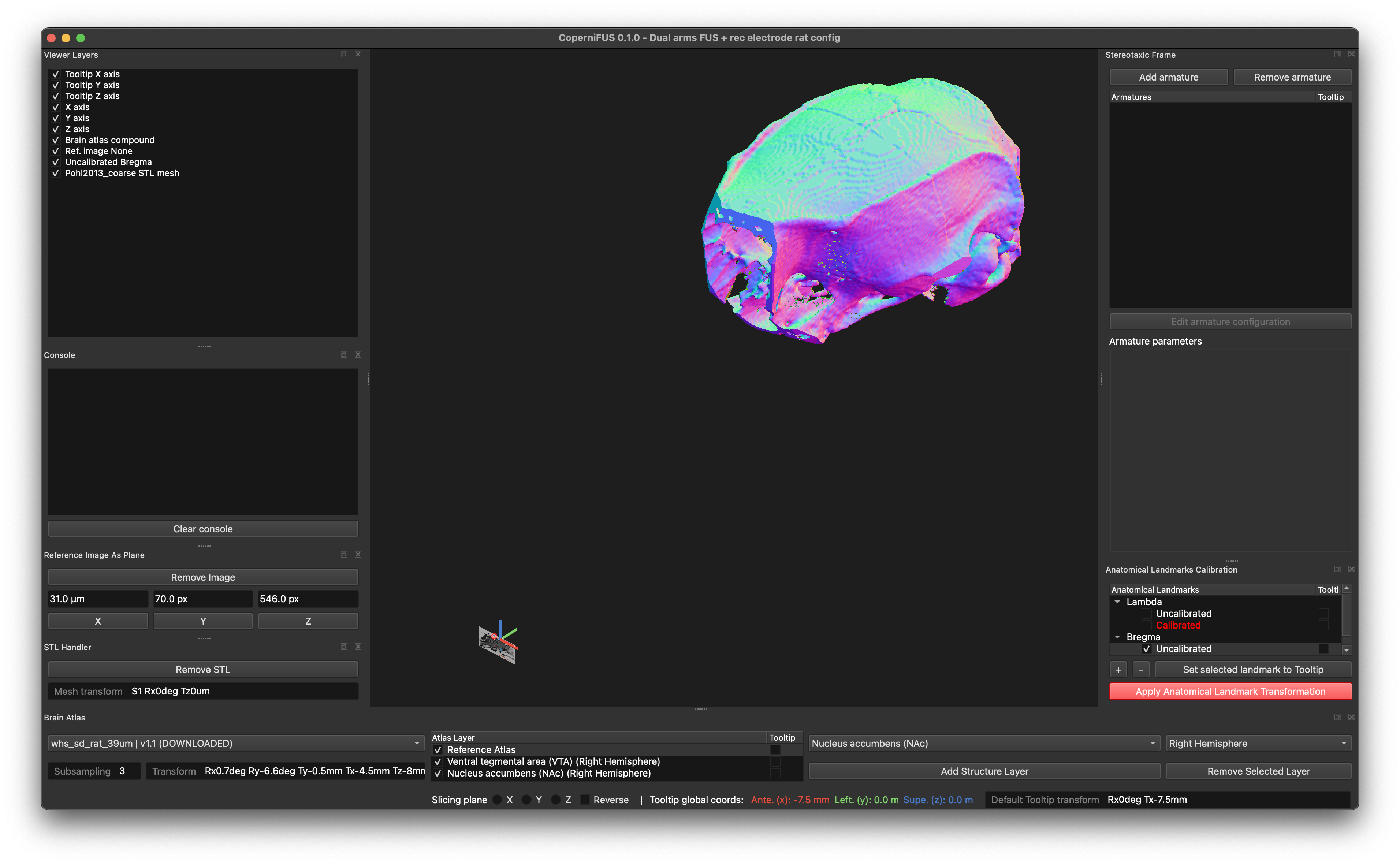
As mentioned, other assets can be registered. Here we will load an stl mesh of a segmented skull [Pohl2013] that will be used for acoustic simulations. To simplify the registration process the mesh will first be loaded using the STL Handler module. Choose the file Pohl2013_coarse.stl provided in the example assets directory.
Note
By default, the mesh is colored based on the face normals orientation. Incidentally, this feature allows the debugging of mesh presenting issues when trying to perform boolean operations.
An appropriate Mesh Transform needs to be determined. Setting a Slicing Plane along the Y axis can simplify this operation. For that, set the Tooltip transform to Ty-1mm and in the Slicing plane section of the status bar select the Y normal.
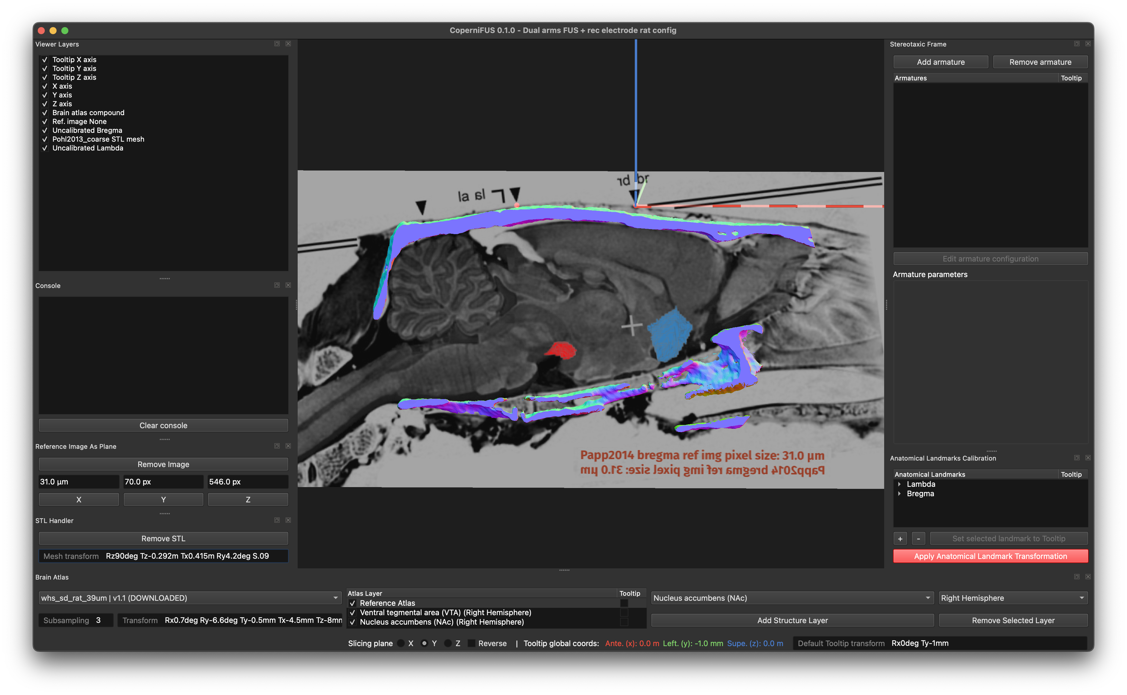
In this example, the following mesh transformation was found: Rz90deg Tz-0.292m Tx0.415m Ry4.2deg S.09 .
4. Add and configure stereotaxic frame Armatures
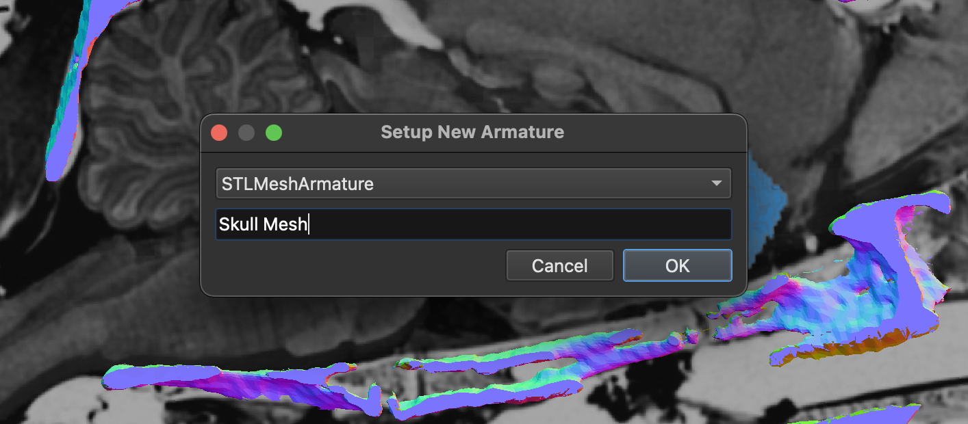
To be used in subsequent operations (mesh boolean, acoustic simulation domain definition, etc.) this mesh needs to be loaded in the Stereotaxic Frame module. To do that click on Add armature and setup an armature of type STLMeshArmature.
Armatures of any types can be configured using the dedicated editor containing an area for constants definition and the actual armature configuration structured in the form of a Python dictionary.
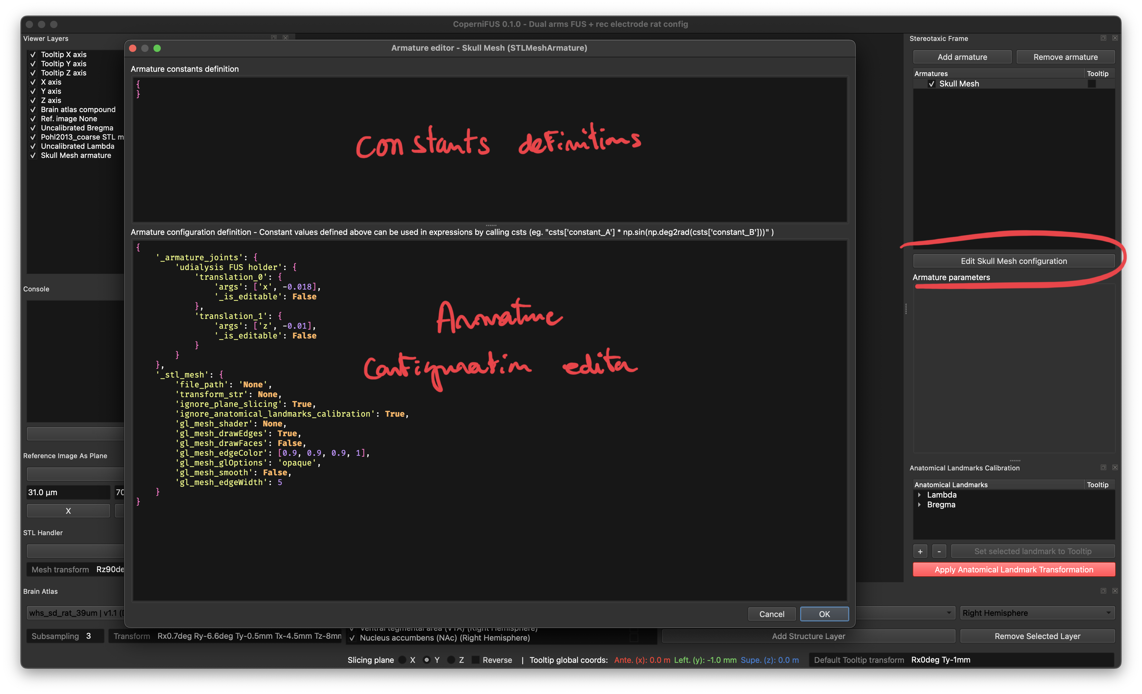
To load the mesh, parameters under the _stl_mesh section need to be edited. The _armature_joints section on the other hand can be discarded in this case. Its purpose will be detailed when defining actual stereotaxic frame elements.
Based on the affine transformation string determined earlier the following configuration can be set.
Note
Armatures reference assets located in a unique directory whose path can be modified at startup using the assets_dir_path argument. If no path is provided, it will default to the CoperniFUS/example/assets directory located in the CoperniFUS source folder.
{
    '_stl_mesh': {
        'file_path': 'Pohl2013_coarse.stl',
        'transform_str': 'Rz90deg Tz-0.292m Tx0.415m Ry4.2deg S.09',
        'ignore_plane_slicing': False,
        'ignore_anatomical_landmarks_calibration': False,
        'gl_mesh_shader': 'boneShader',
        'gl_mesh_drawEdges': False,
        'gl_mesh_drawFaces': True,
        'gl_mesh_edgeColor': [0.9, 0.9, 0.9, 0.7],
        'gl_mesh_glOptions': 'opaque',
        'gl_mesh_smooth': False,
        'gl_mesh_edgeWidth': 2
    }
}
At this point the mesh loaded in the STL Handler module can be removed. Note that armature visibility and Tooltip location inheritance can be set in the Stereotaxic Frame module in the same fashion as in the Brain Atlas and Anatomical Landmarks Calibration modules.
For demonstration purposes we will now add Stereotaxic Armatures that would be used for the planing of an experiment where focused ultrasound (FUS) is applied to the VTA while monitoring the activity of the NAc region using a recording electrode.
To reference anatomical coordinates on the animal during the experiment, we will first define a dummy probe with a needle tip. As mentioned in Armature definition procedure, careful measurement of all stereotaxic elements needs to be performed to obtain accurate planning and simulation results. For reference, an armature definition validation procedure is also described in the Armature definition procedure section.
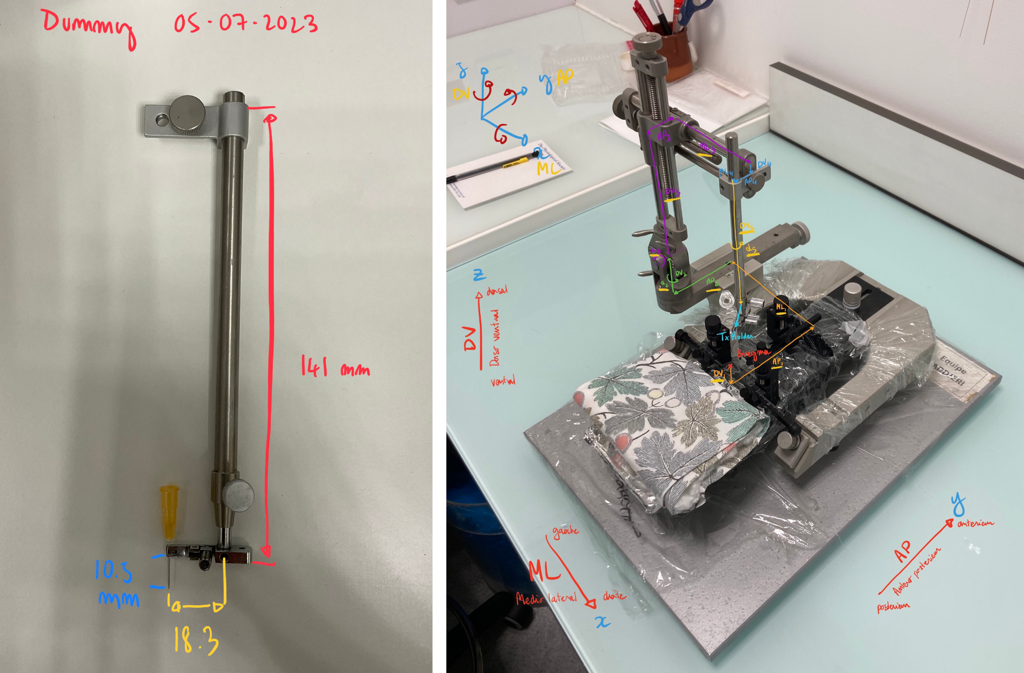
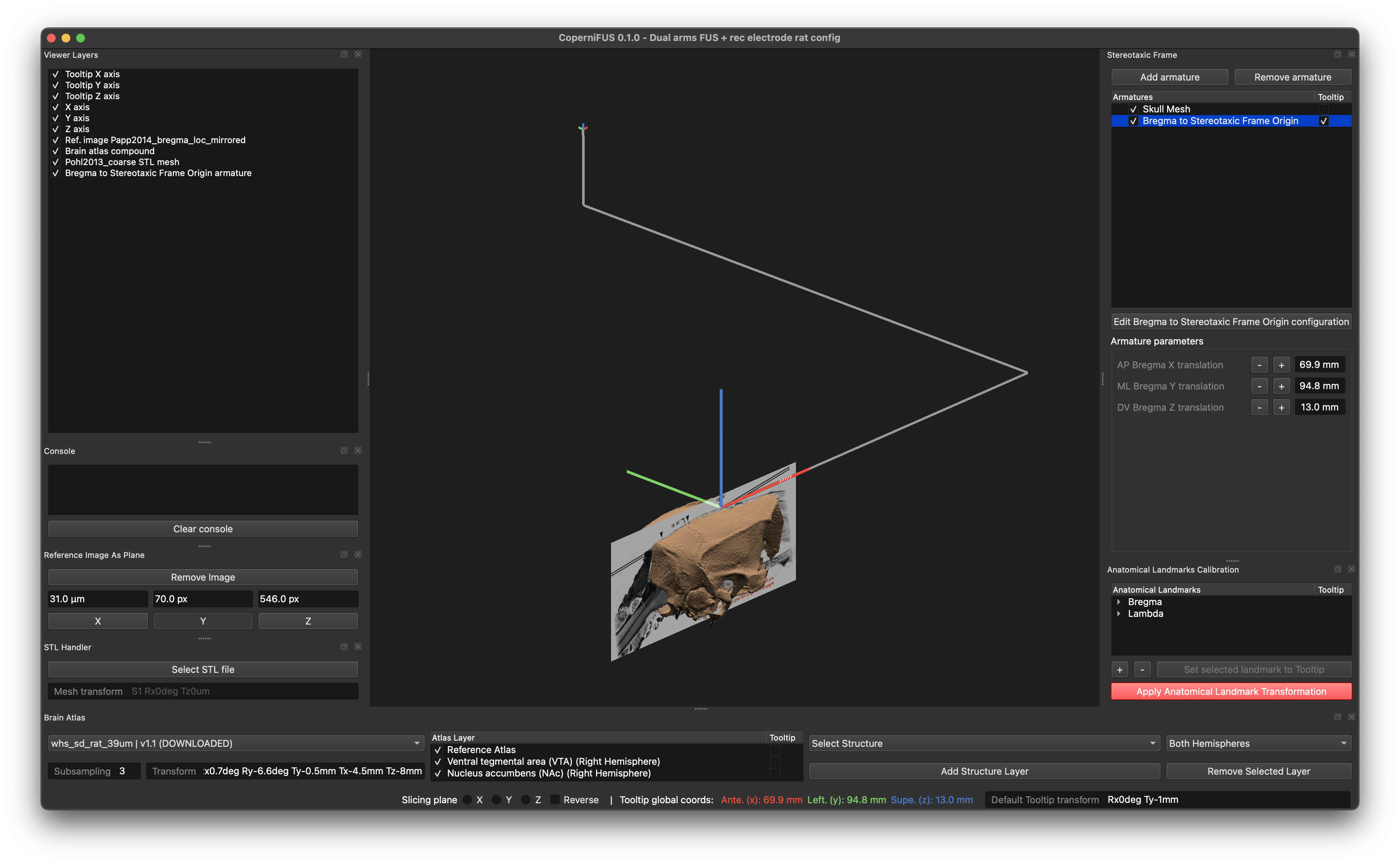
As we touched on earlier, Stereotaxic Frame joints are defined in the _armature_joints section of the armature configuration dictionary. To start, we will define the location of the stereotaxic frame origin relative to the spatial reference we choose, which is the Bregma landmark in this example. To that end, a regular Armature named Bregma to Stereotaxic Frame Origin is created by pressing the Add armature button. Translations along X, Y and Z need to be defined. Furthermore, the location of Bregma relative to the frame origin will likely be specific to each animals included in the study, we thus want to make these parameters easily editable.
Armature joints are defined in the following way
{
    '_armature_joints': {
        'Name of an editable joint: {
            'translation_0': {                  # Transformation identifier -> both translation_x and translation_x can be defined. Note that multiple transformations can be defined for a single joint. Simply make sure that their identifiers are unique. Use integers to that end (eg. translation_0, translation_1, etc.)
                'args': ['x', 0.05],            # Transformation arguments: in the case of _armature_joints, an axis string ('x', 'y', 'z')  followed the transformation value need to be specified. As demonstrated bellow, expressions referencing  constants defined in the constants section of the editor can also be given.
                '_is_editable': True,           # Choose wether this parameter can edited in the GUI
                '_force_gui_location_to': 3,        # For editable parameters, the order of widgets can be altered by specifying and int
                '_edit_increment': 0.0005,          # For editable parameters, increments applied when pressing the +/- buttons can be set here.
                '_unit': 'm'                                        # For editable parameters, a unit suffix (usually 'm' or 'deg') can be specified
        '_color': 'x_RED',                                  # For editable parameters, a color can be specified. x_RED, y_GREEN and z_BLUE are reserved names matching axes colors shown throughout the GUI.

            }
        },
        'ML Bregma': {
            'rotation_0': {
                'args': ['y', "csts['alpha'] * 2”], # Constants defined in the constants section of the editor are referenced csts['constant_name']
                '_is_editable': False,
            }
        }
    }
}
In the context of the Bregma to Stereotaxic Frame Origin armature, default demonstration constants can be deleted and the configuration can be set to:
{
    '_armature_joints': {
        'AP Bregma': {
            'translation_0': {
                'args': ['x', 0.0699],
                '_is_editable': True,
                '_edit_increment': 0.0005,
                '_color': 'x_RED',
                '_unit': 'm'
            }
        },
        'ML Bregma': {
            'translation_0': {
                'args': ['y', 0.0948],
                '_is_editable': True,
                '_edit_increment': 0.0005,
                '_color': 'y_GREEN',
                '_unit': 'm'
            }
        },
        'DV Bregma': {
            'translation_0': {
                'args': ['z', 0.013],
                '_is_editable': True,
                '_edit_increment': 0.0005,
                '_color': 'z_BLUE',
                '_unit': 'm'
            }
        }
    }
}
After application of the configuration, a wireframe armature can be made visible in the viewer.
The rest of the registration probe can be defined as a set of three armatures: 1. a stereotaxic frame Arm with linkages adjustable with dials, 2. a Probe Shaft with a fixed length but a rotational degree of freedom along z and 3. the Probe Tip which has fixed dimensions.
1. Coordinates Registration Probe Arm (type: Armature)
Constants:
{
    'L1': 0.0215,
    'L2': 0.135,
    'L3': 0.0483,
    'L4': 0.077,
    'L5': 0.0245,
    'L6': 0.1152,
    'L7': 0.013,
    'L8': 0.0303,
    'L9': 0.014,
    'L10': 0.0053,
    'L11': 0.0128,
    'L12': 0.136,
    'L13': 0.0245,
    'L14': 0.014,
    'd1': 0.0332,
    'd2': 0.0095,
    'd3': 0.0096,
    'd4': 0.008
}
Configuration dictionary:
{
    '_armature_joints': {
        'ML0': {
            'translation_0': {
                'args': ['y', "csts['L1']/2"],
                '_is_editable': False
            }
        },
        'AP Knob': {
            'translation_0': {
                'args': ['x', 0.0595],
                '_is_editable': True,
                '_force_gui_location_to': 0,
                '_edit_increment': 0.0005,
                '_color': 'x_RED',
                '_unit': 'm'
            }
        },
        'AP0': {
            'translation_0': {
                'args': ['x', "-csts['L2'] + csts['d1']/2"],
                '_is_editable': False
            }
        },
        'DV0': {
            'translation_0': {
                'args': ['z', "csts['L3'] - csts['d2']/2"],
                '_is_editable': False
            },
            'rotation_0': {
                'args': ['z', 0.0, 'degrees'],
                '_is_editable': True,
                '_edit_increment': 1,
                '_unit': 'deg'
            }
        },
        'DV1': {
            'translation_0': {
                'args': ['z', "csts['d2']/2 + csts['L4'] - csts['L5']"],
                '_is_editable': False
            },
            'rotation_0': {
                'args': ['x', 0.0, 'degrees'],
                '_is_editable': True,
                '_edit_increment': 1,
                '_unit': 'deg'
            }
        },
        'DV Knob': {
            'translation_0': {
                'args': ['z', 0.0258],
                '_is_editable': True,
                '_force_gui_location_to': 2,
                '_color': 'z_BLUE',
                '_edit_increment': 0.0005,
                '_unit': 'm'
            }
        },
        'ML Knob': {
            'translation_0': {
                'args': ['y', 0.0185],
                '_is_editable': True,
                '_force_gui_location_to': 1,
                '_edit_increment': 0.0005,
                '_color': 'y_GREEN',
                '_unit': 'm'
            }
        },
        'AP2': {
            'translation_0': {
                'args': ['x', "csts['d3']/2 - csts['L7'] + csts['L8'] - csts['L9'] - csts['L10'] - csts['d4']/2"],
                '_is_editable': False
            }
        },
        'ML2': {
            'translation_0': {
                'args': ['y', "-csts['d3']/2 + csts['L11'] - csts['L12'] + csts['d4']/2"],
                '_is_editable': False
            }
        },
        'DV2': {
            'translation_0': {
                'args': ['z', "csts['L13'] - csts['L14']"],
                '_is_editable': False
            }
        }
    }
}
2. Coords Registration Probe Shaft (type: Armature)
Constants:
{
    'registration_shaft_len': 0.1337,
}
Configuration dictionary:
{
    '_armature_joints': {
        'Registration probe shaft': {
            'translation_0': {
                'args': ['z', "- csts['registration_shaft_len']"],
                '_is_editable': False,
            },
            'rotation_0': {
                'args': ['z', 0, 'degrees'],
                '_is_editable': True,
                '_edit_increment': 1,
                '_unit': 'deg'
            },
            'rotation_1': {
                'args': ['x', 0, 'degrees'],
                '_is_editable': True,
                '_edit_increment': 1,
                '_unit': 'deg'
            }
        }
    }
}
3. Coords Registration Probe Tip (type: Armature)
Constants:
{
    'registration_tip_x_offset': 0.0183,
    'registration_tip_z_height': 0.0164
}
Configuration dictionary:
{
    '_armature_joints': {
        'Registration probe tip offset': {
            'translation_0': {
                'args': ['x', "- csts['registration_tip_x_offset']"],
                '_is_editable': False,
            }
        },
        'Registration probe tip length': {
            'translation_0': {
                'args': ['z', "- csts['registration_tip_z_height']"],
                '_is_editable': False,
            }
        }
    }
}
After creation, created armatures need to be assembled.
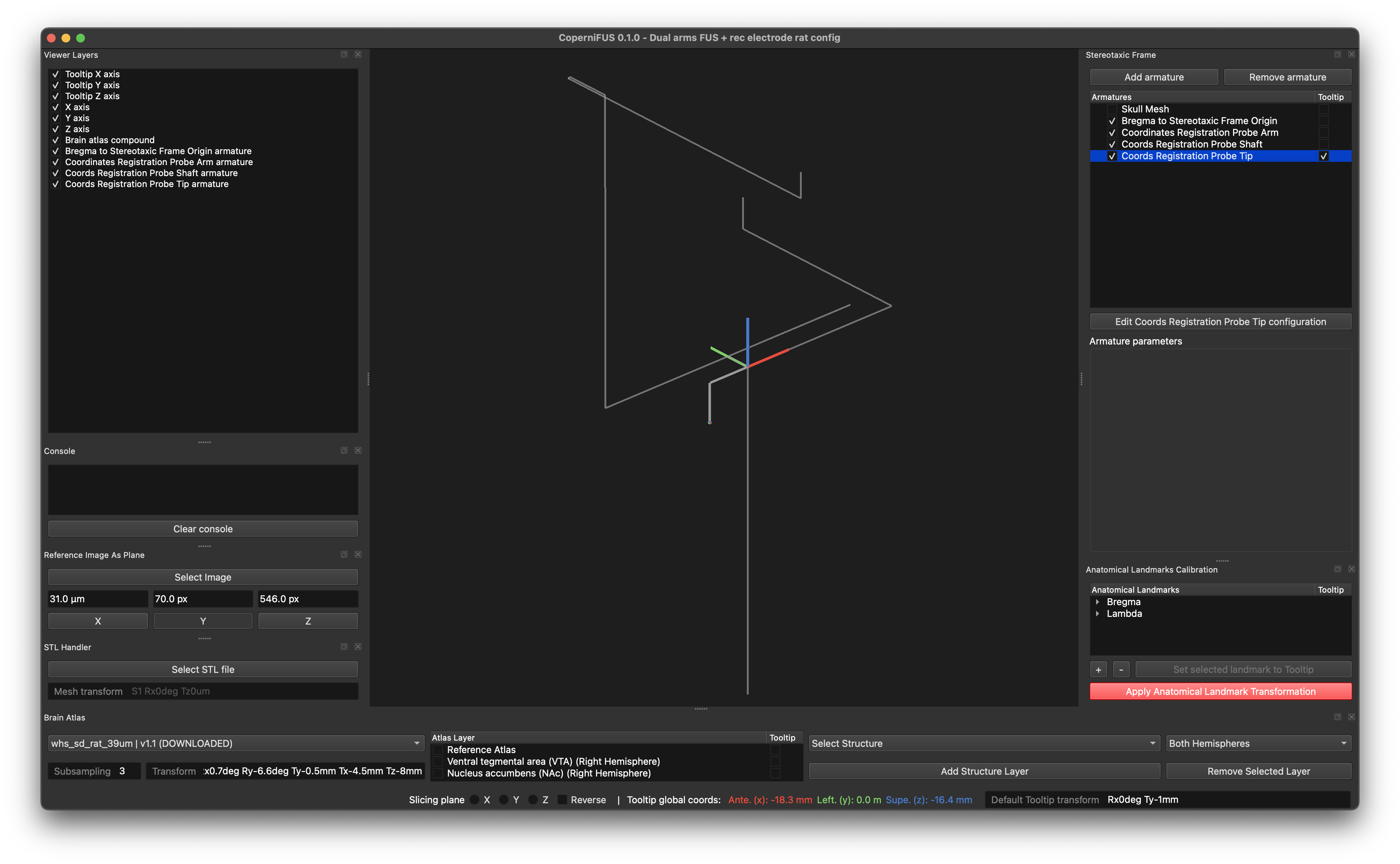
Using the armature inheritance feature, stereotaxic architectures can be set via drag and drop:
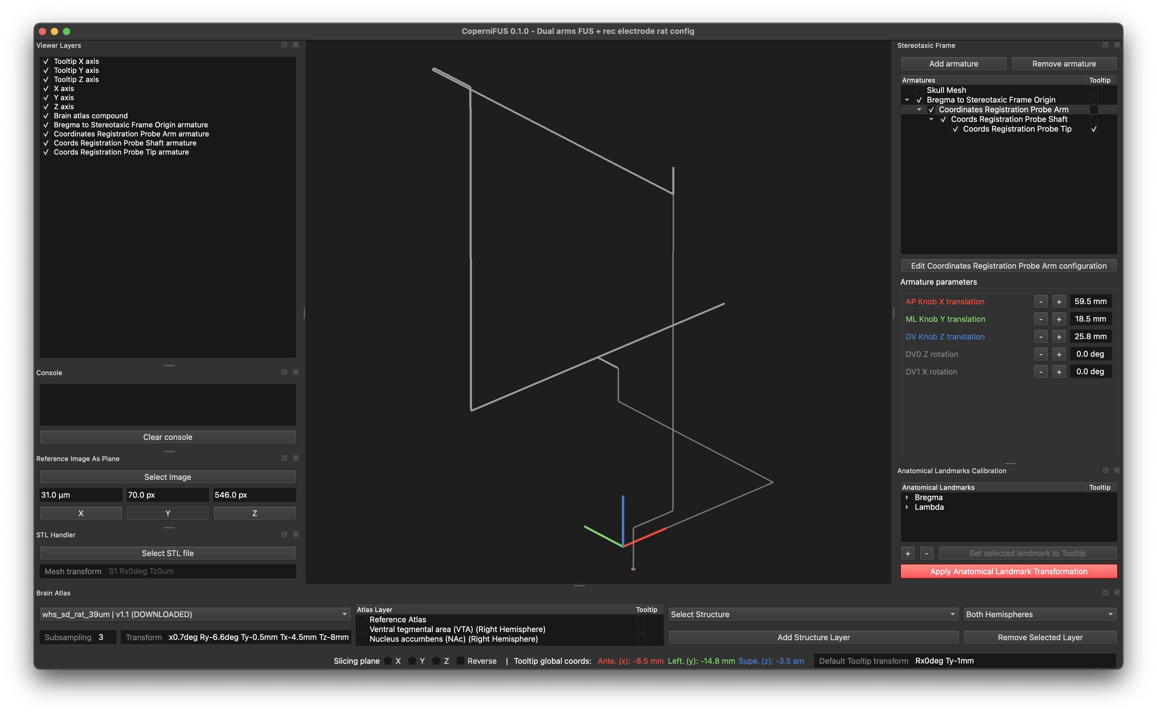
Using this system, on experiment day, the dummy probe modeled for coordinate registration purposes can be mounted on the frame and aligned on the Bregma structure of the animal. Values dialed on the frame arm can be reported in CoperniFUS.
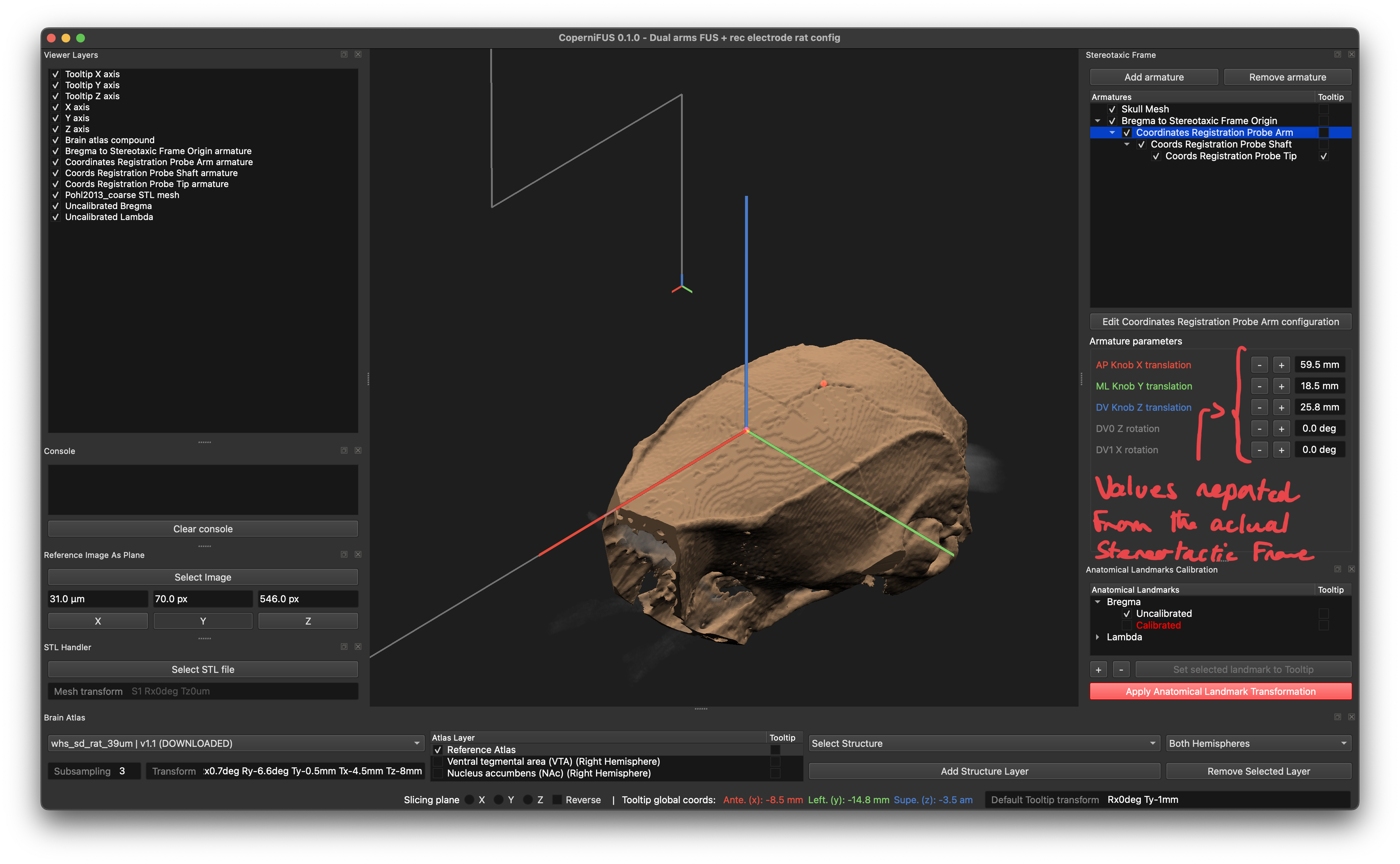
In the software, parameters of the Bregma to Stereotaxic Frame Origin armature can then be adjusted so that the modeled tip aligns with the origin of the coordinate system (Bregma).
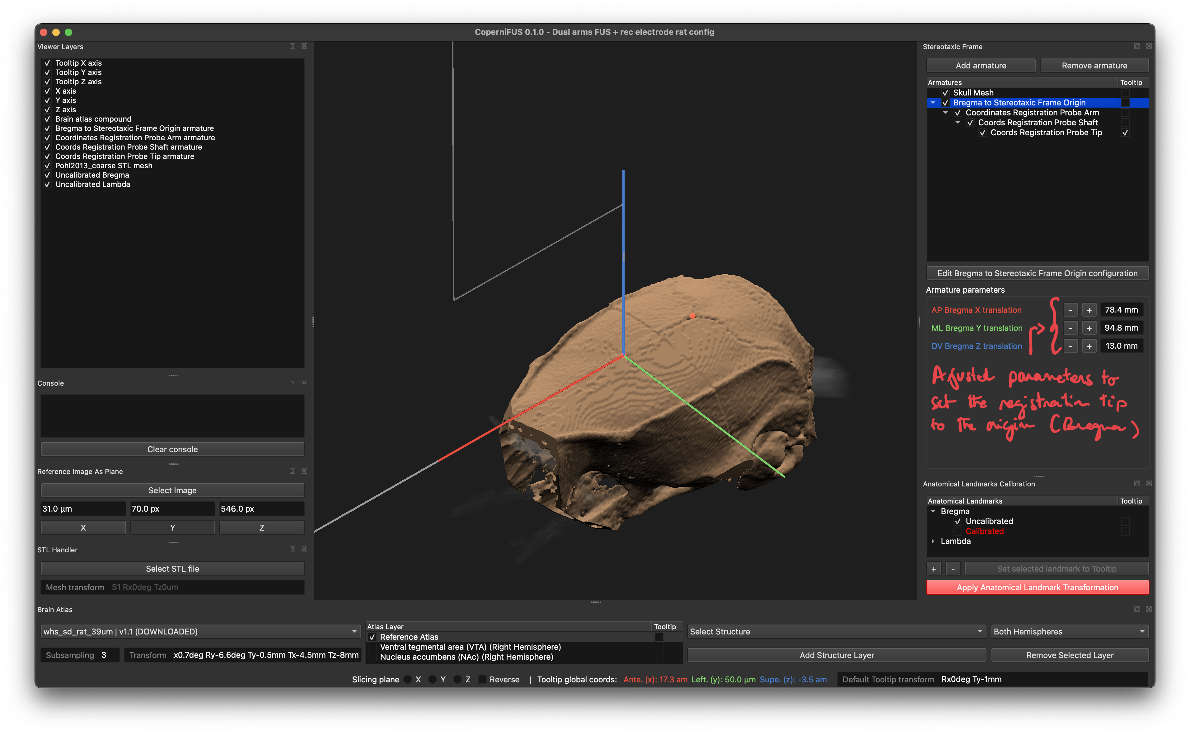
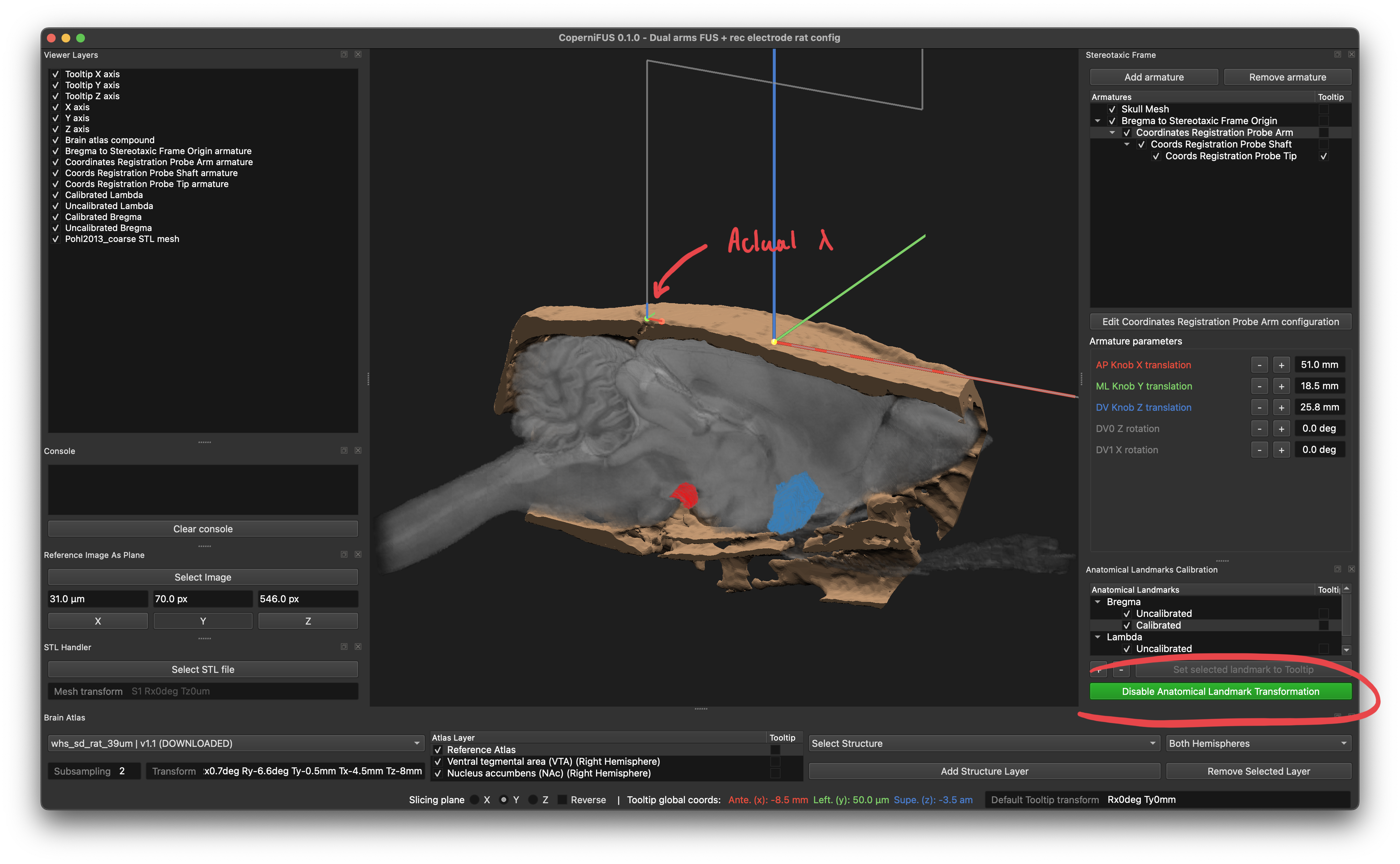
The operation can be reproduced for the Lambda landmark. After setting the Tooltip on the Registration Probe Tip, the location of the calibrated landmark can be set.
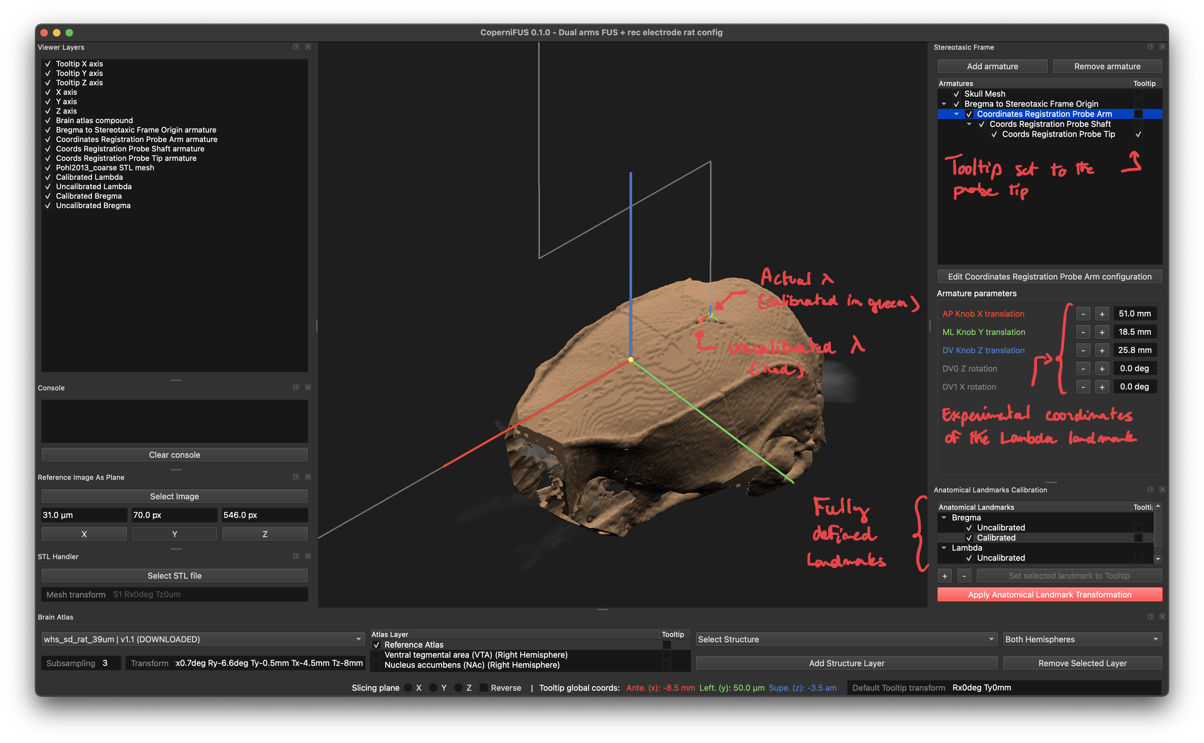
Once all Anatomical Landmarks are defined, calibration can be performed by clicking on Apply Anatomical Landmark Transformation.
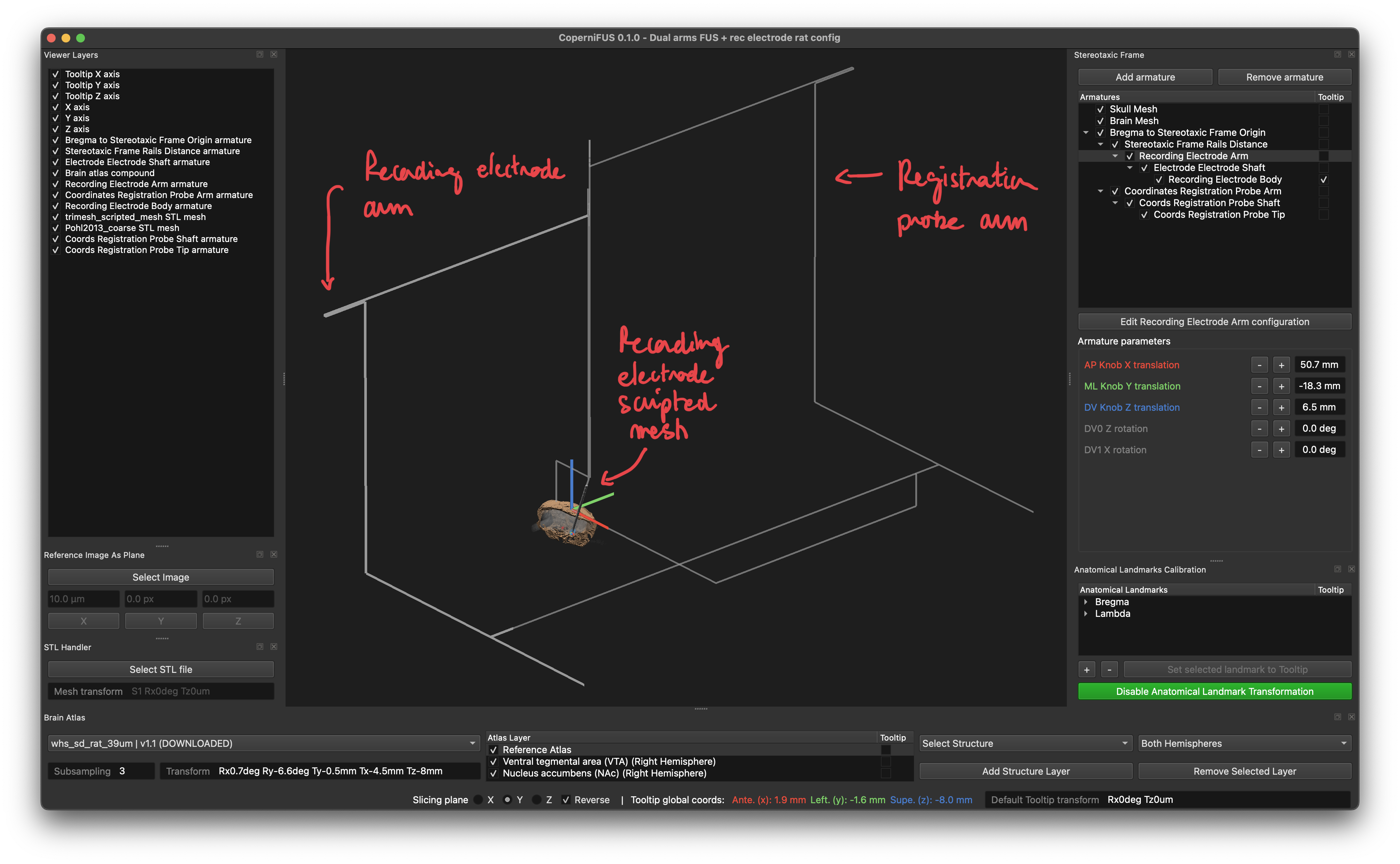
Let us now introduce an other type of armature allowing the creation of meshes using the trimesh scripting syntax.
A second stereotaxic frame arm is first defined.
Note
For the sake of legibility configuration dictionaries will not be systematically provided in this tutorial. You can nevertheless load the complete configuration file provided in the example folder.
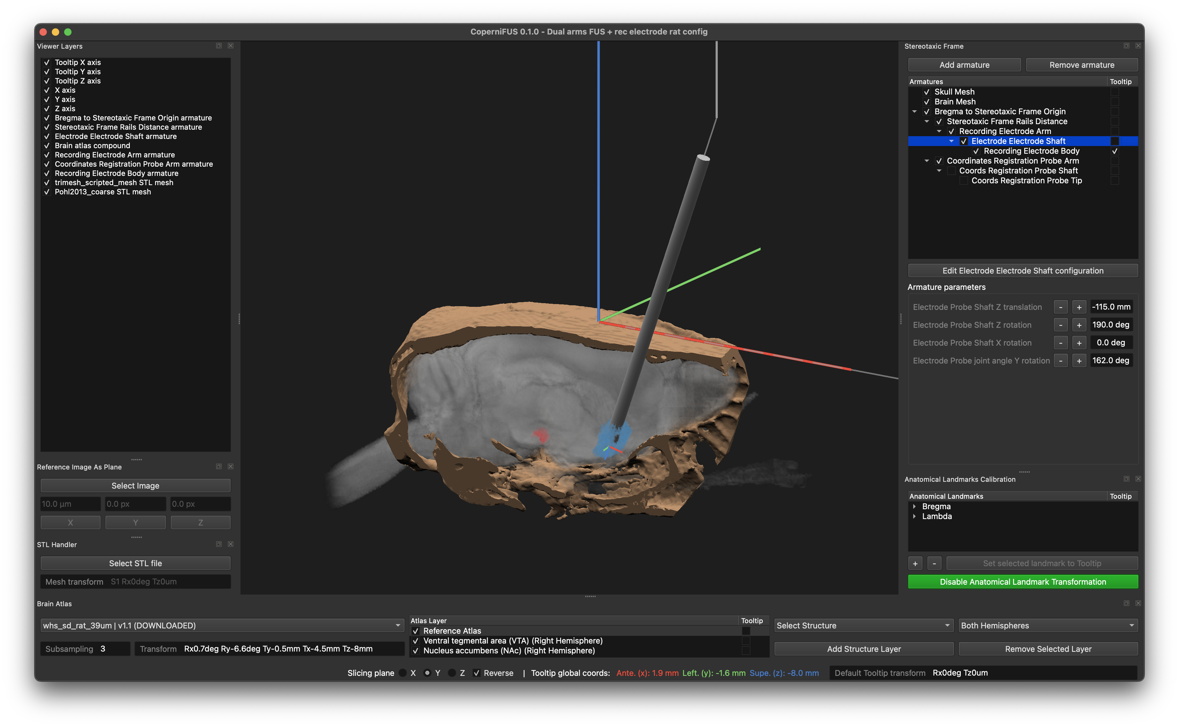
For demonstration sakes, we modelled the body of the recording electrode by specifying the following trimesh script in the _trimesh_script section of the armature configuration dictionary.
'_trimesh_script': """
path_2d = trimesh.path.creation.circle(radius=probe_diameter/2, segments=8)
extrusion = path_2d.extrude(-probe_length)
mesh = extrusion.to_mesh()
“””
> Upon execution, the script must define a mesh object.
To facilitate the edition of geometry parameters, _trimesh_script_coords can be defined using the syntax presented for editable armature joint definition.
'_trimesh_script_coords': {
    'probe_diameter': {
        'args': ['diameter', 0.0009],
        '_is_editable': True,
        '_edit_increment': 0.0005,
        '_param_label': 'Probe Mesh diameter',
        '_color': 'grey',
        '_unit': 'm'
    },
    'probe_length': {
        'args': ['length', 0.022],
        '_is_editable': True,
        '_edit_increment': 0.0005,
        '_param_label': 'Probe Mesh length',
        '_color': 'grey',
        '_unit': 'm'
    }
}
5. Setting up and running k-wave simulations
Mobilizing all the concepts introduced up to this point, a last stereotaxic arm supporting a focused ultrasound transducer (FUS) can be defined.
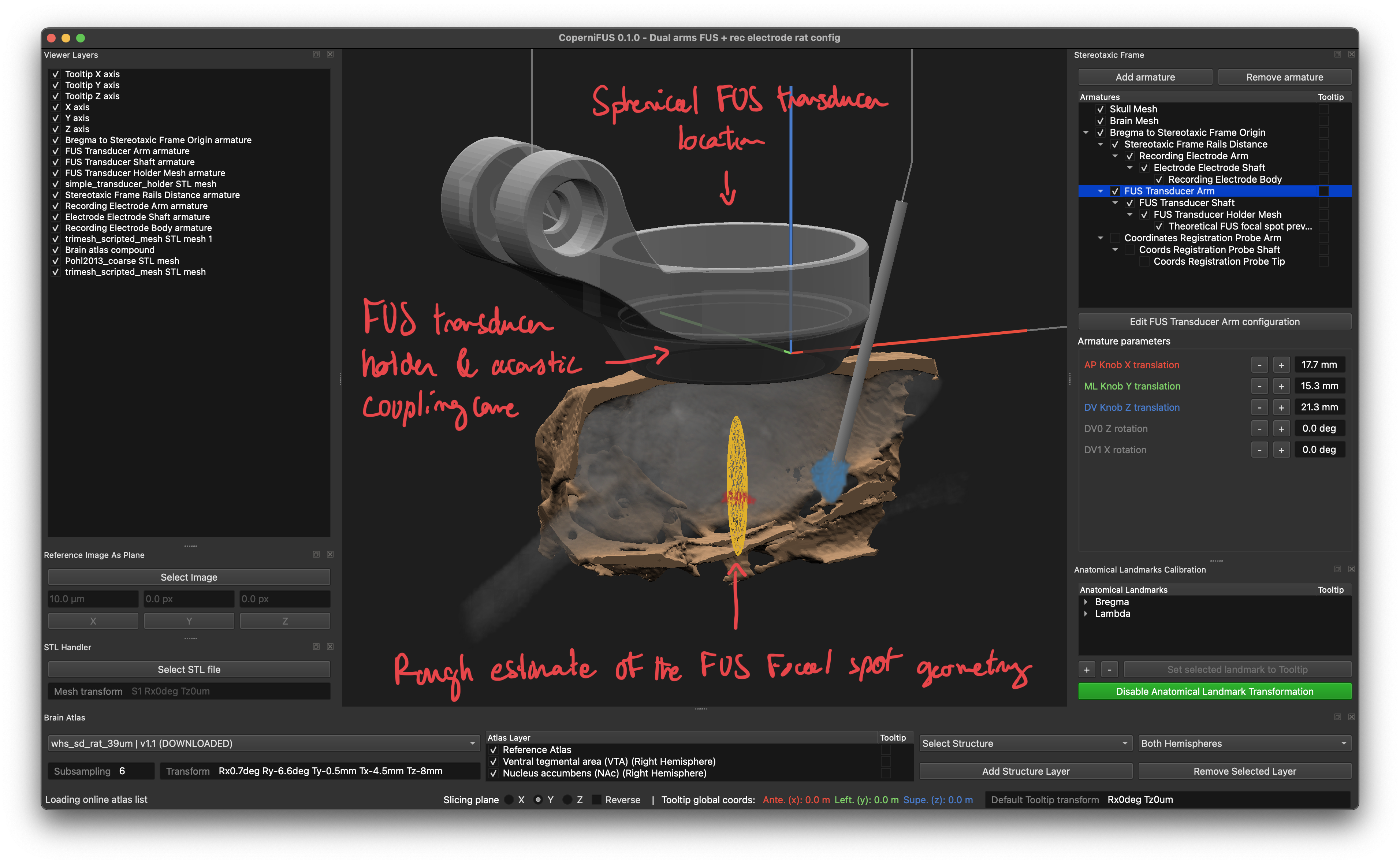
A TrimeshScriptArmature is once again used to preview a rough approximation of the FUS focal spot location. Even though this geometry does not take aberration introduced by the skull into account , it allows to make first guesses on the optimal stereotaxic frame arrangement and anticipate potential spatial constraints.
'_trimesh_script': """

c0 = 1500
lambd = c0 / tx_freq
len_focus = 7*lambd * (F_tx/D_tx)**2
width_focus = (lambd * F_tx) / D_tx
fspot_est_zloc = np.sqrt(F_tx**2 - (D_tx / 2)**2)
mesh = trimesh.creation.icosphere(radius=1, subsivisions=1)
mesh.apply_scale((width_focus, width_focus, len_focus))
mesh.apply_translation((0, 0, -fspot_est_zloc))

"""
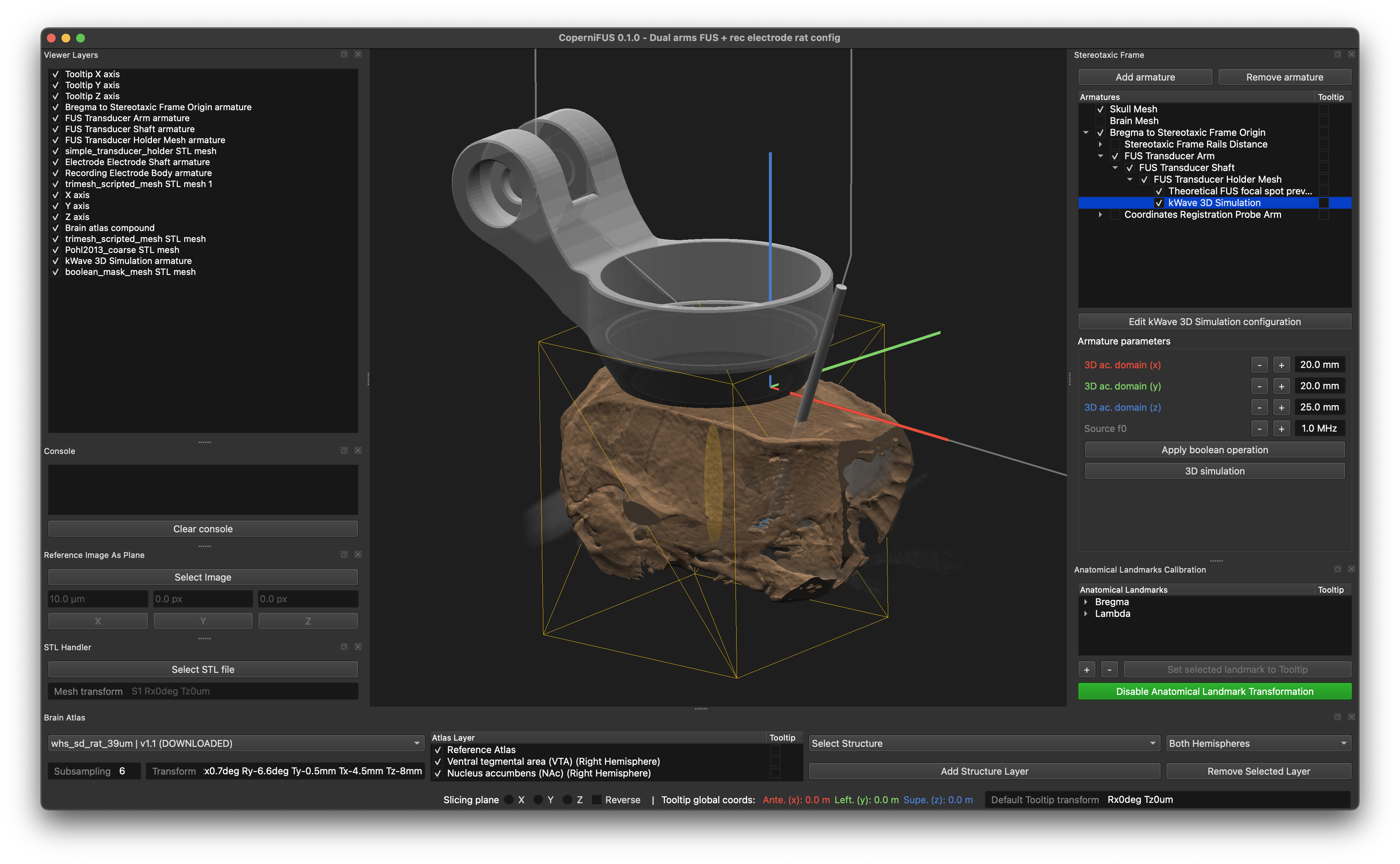
To conduct k-wave acoustic simulations and evaluate the effect of the skull on the ultrasound field a new KWave3dSimulationArmature can be defined. Under the hood, KWave3dSimulationArmature objects inherit properties from STLMeshBooleanArmature, using a trimesh script a cuboid mesh is created and loaded in the viewer indicating the dimensions of the simulation domain. In the coming steps, we will see how this mesh is also used to compute the intersection of the domain with other mesh armatures loaded in CoperniFUS allowing the definition of maps of acoustic material properties, that will eventually be forwarded to k-wave when running simulations.
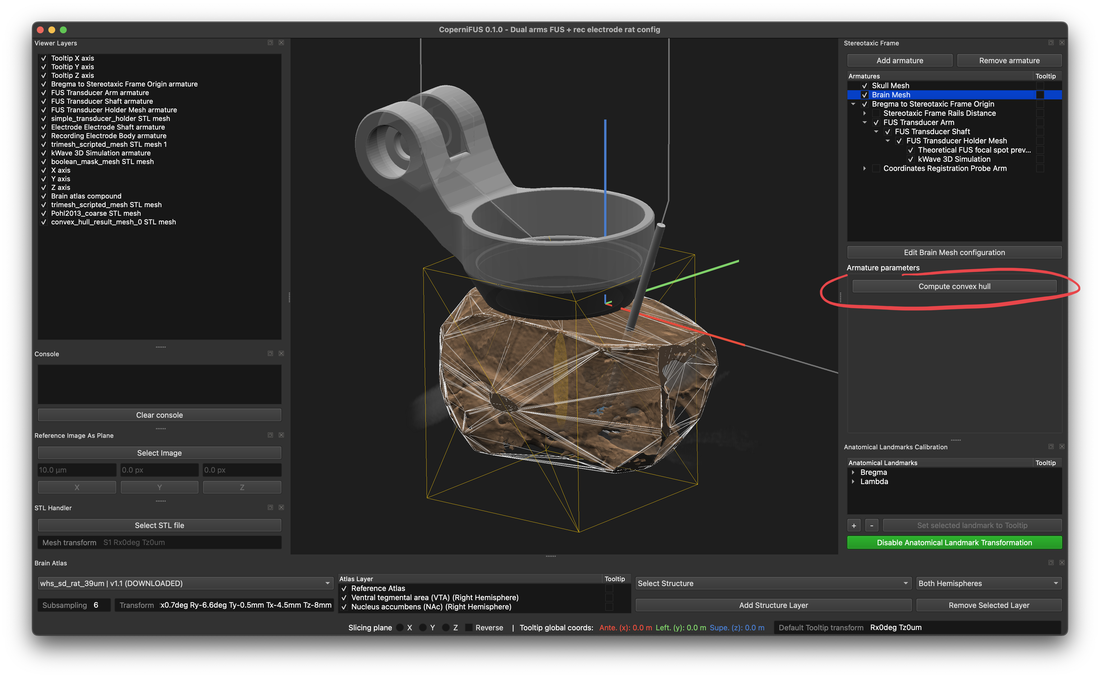
However to properly describe the acoustic properties of the domain, a last mesh meeds to be defined. In deed, by default, the assumption is made that the whole domain is composed of water. From the current loaded assets, acoustic skull properties can be assigned to intersections of the domain with the Skull Mesh armature. We however need to create a last mesh to assign brain tissues properties to the inside of the skull. As a first approach, a convex hull mesh can be created based on the skull mesh. This can easily be done using an STLMeshConvexHull armature and specify the name of the Skull Mesh armature as the _src_mesh under the _convex_hull section of the configuration dictionary.
{
    '_stl_mesh': {
        'file_path': 'None',
        'transform_str': 'S1 Rx0deg Tz0mm',
        'ignore_plane_slicing': False,
        'ignore_anatomical_landmarks_calibration': True,
        'gl_mesh_shader': None,
        'gl_mesh_drawEdges': True,
        'gl_mesh_drawFaces': False,
        'gl_mesh_edgeColor': [0.9, 0.9, 0.9, 1],
        'gl_mesh_glOptions': 'opaque',
        'gl_mesh_smooth': False,
        'gl_mesh_edgeWidth': 5
    },
    '_convex_hull': {
        '_src_mesh': 'Skull Mesh',
        'ignore_plane_slicing': True,
        '_mask_preview_gl_options': {
            'gl_mesh_shader': None,
            'gl_mesh_drawEdges': True,
            'gl_mesh_drawFaces': False,
            'gl_mesh_edgeColor': [0.5, 0, 0, 1],
            'gl_mesh_glOptions': 'opaque',
            'gl_mesh_smooth': False,
            'gl_mesh_edgeWidth': 5
        }
    }
}
In the kWave 3D Simulation armature, references of the mesh armatures used for computation of the domain intersection using boolean operations can be specified in the _boolean_mask section:
'_boolean_mask': {
    '_boolean_operations': {
        '1': ['intersection', ['Brain Mesh', '_boolean_mask']],
        '2': ['intersection', ['Skull Mesh', '_boolean_mask']]
    },
Boolean operations indices used match the suffixes of acoustic parameters defined in _3dcartesian_domain_acoustic_params:
'_3dcartesian_domain_acoustic_params': {
    'c_0': 1482.3,          # Water everywhere (0 index)
    'rho_0': 994.04,
    'alpha_0': 0.0022,
    'alpha_power_0': 1.0,
    'c_1': 1546,            # Brain tissue properties inside the boolean intersection mesh with index '1'
    'rho_1': 1045,
    'alpha_1': 0.208,
    'alpha_power_1': 1.3,
    'c_2': 2400,            # Skull properties inside the boolean intersection mesh with index '2'
    'rho_2': 1850,
    'alpha_2': 2.693,
    'alpha_power_2': 1.18,
    ...
}
Note
Also note that the order of operations matters as first material assignments will be overridden by later ones. In this example, brain tissues properties are overridden by skull properties.
At this point mesh intersections can be computed (make sure that all the meshes involved like the skull convex hull have been computed),
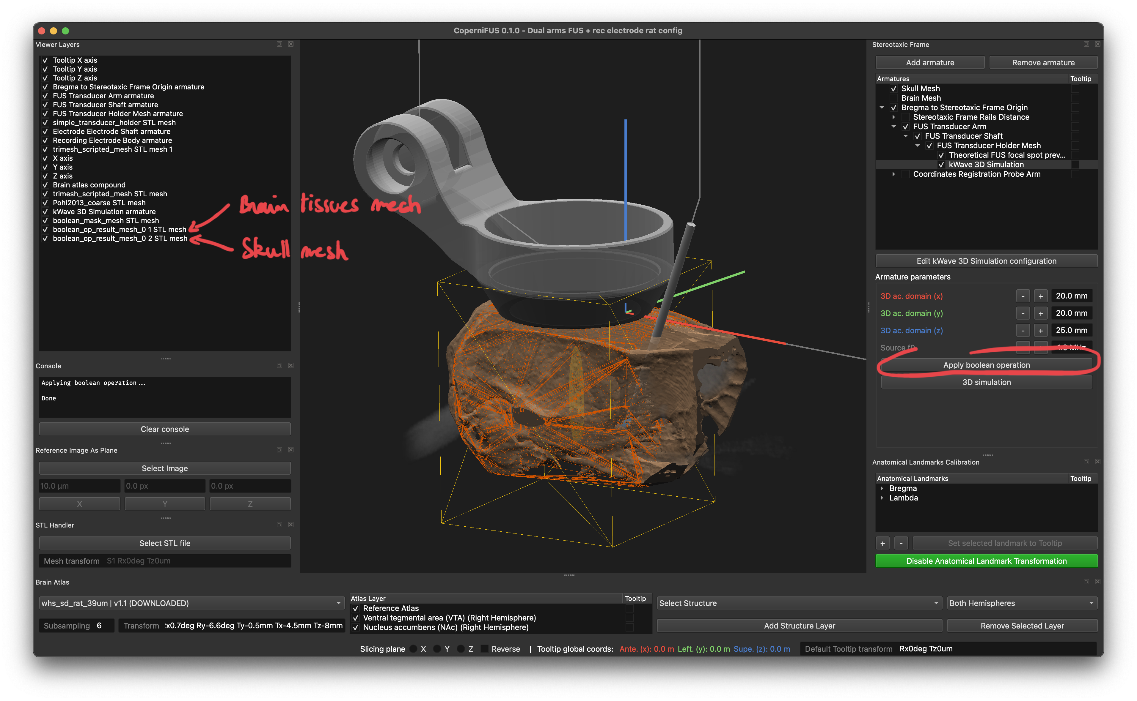
and the simulation initiated.
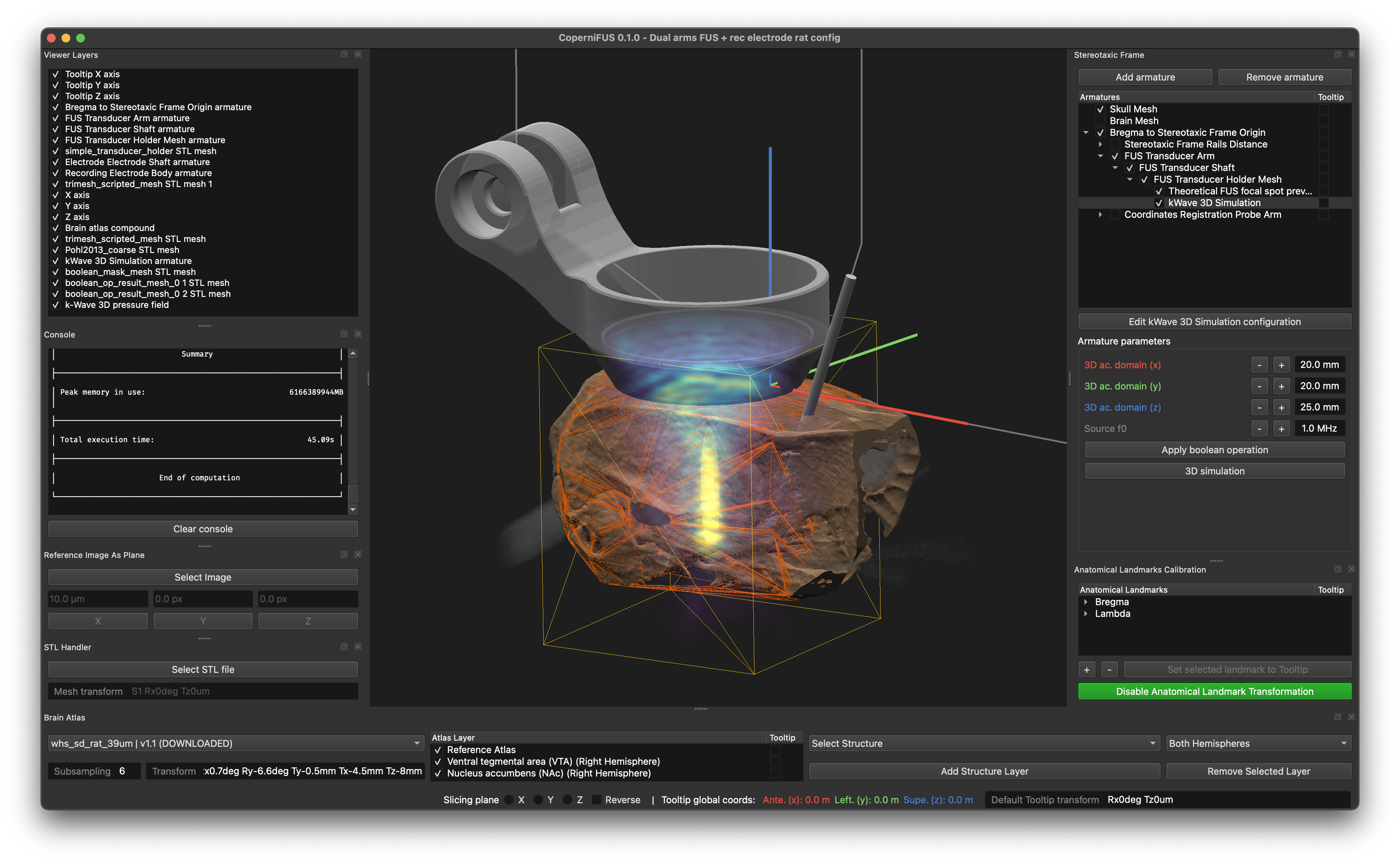
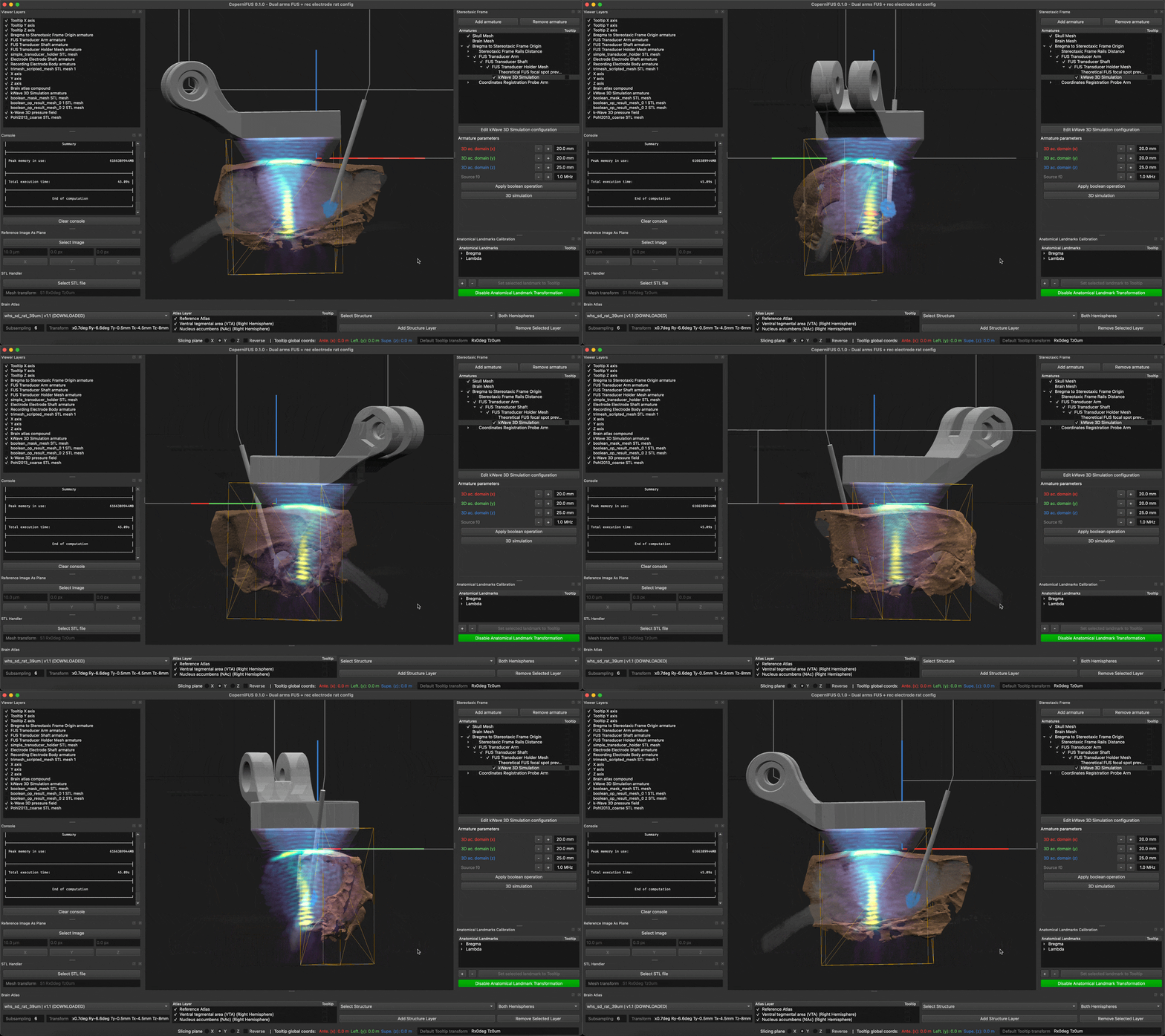
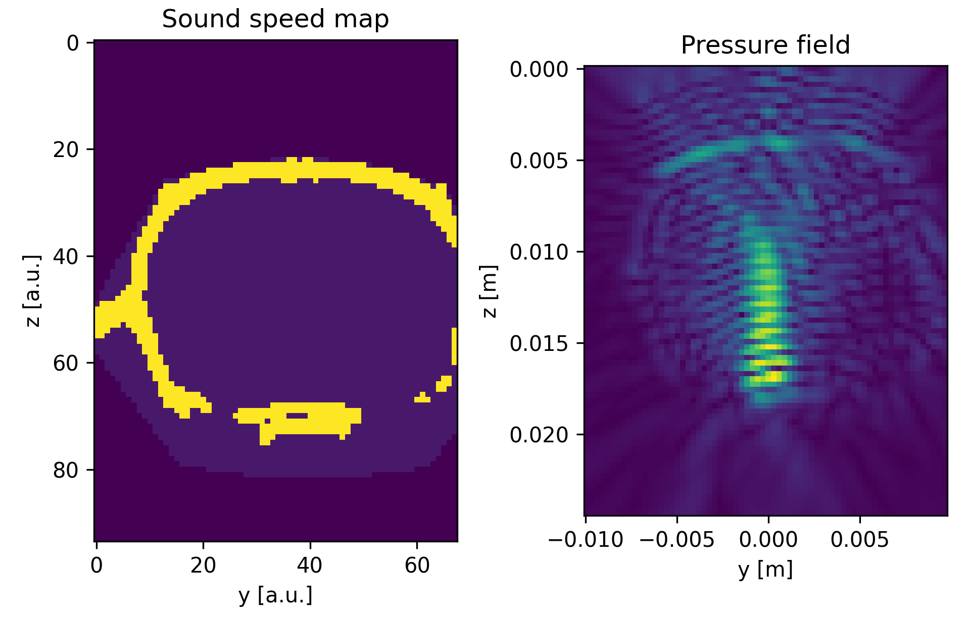
If running CoperniFUS in interactive mode, simulation results can be grabbed for further analyses.
cfv = coperniFUSviewer(
    disable_internal_console=False,
)

stereotaxic_frame_handle = cfv.get_module_object_from_name('StereotaxicFrame')
acsim_armature = stereotaxic_frame_handle.armatures_objects['kWave 3D Simulation']

import matplotlib.pyplot as plt

p_amp_xyz, x, y, z = acsim_armature.kw3D.p_amp_xyz

fig, axs = plt.subplots(ncols=2)
axs[0].imshow(acsim_armature.kw3D.medium.sound_speed[34].T)
axs[0].set_title('Sound speed map')
axs[0].set_xlabel('y [a.u.]')
axs[0].set_ylabel('z [a.u.]')

axs[1].imshow(p_amp_xyz[34].T, extent=[y[0], y[-1], z[-1], z[0]])
axs[1].set_title('Pressure field')
axs[1].set_xlabel('y [m]')
axs[1].set_ylabel('z [m]')